Chapter: Modern Analytical Chemistry: Titrimetric Methods of Analysis
Acid–Base Titration Curves
Acid–Base Titration Curves
In
the overview we noted that the experimentally determined end point should coincide with the titration’s equivalence point. For an acid–base
titra- tion, the equivalence point is characterized by a pH level that
is a function of the acid–base strengths and concentrations of the analyte
and titrant. The pH at the end point, however, may or may not correspond to the pH at the equivalence point.
To understand the relationship between end points and equivalence points
we must know how the pH changes
during a titration. In this section
we will learn
how to construct titration
curves for several important types of acid–base titrations.
Titrating Strong Acids and Strong Bases
For our first
titration curve let’s
consider the titration of 50.0 mL of 0.100
M HCl with 0.200 M NaOH. For the reaction
of a strong base
with a strong
acid the only
equilibrium reaction of importance is
H3O+(aq)+ OH–(aq)
< = = > 2H2O(l) 9.1
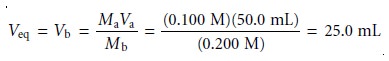
The
first task in constructing the titration curve
is to calculate the volume
of NaOH needed to reach the equivalence point.
At the equivalence point we know from re-
action 9.1 that
Moles HCl = moles NaOH
or
MaVa = MbVb
where the subscript ‘a’ indicates the acid, HCl, and the subscript ‘b’ indicates the base, NaOH. The volume
of NaOH needed
to reach the equivalence point,
there- fore, is
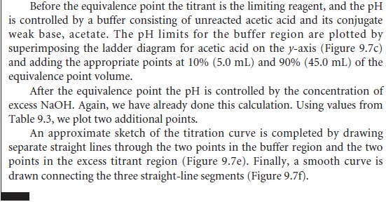
Before the equivalence point, HCl is present in excess and the pH is determined by the concentration of excess HCl. Initially the solution is 0.100 M in HCl, which,
since HCl is a strong
acid, means that
the pH is
pH
= –log[H3O+] = –log[HCl] = –log(0.100) = 1.00
The equilibrium constant
for reaction 9.1 is (Kw)–1, or 1.00 x 10¹⁴. Since this is such
a large value we can treat reaction
9.1 as though it goes to completion. After adding 10.0 mL
of NaOH, therefore, the concentration of excess HCl is
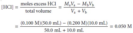
giving a pH of 1.30.
At
the equivalence point
the moles of HCl and the moles
of NaOH are equal.
Since neither the acid nor the base is in excess, the pH is determined by the dissoci- ation of water.
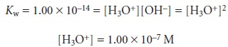
Thus, the pH at the equivalence point is 7.00.
Finally, for volumes
of NaOH greater
than the equivalence point volume, the pH
is determined by the concentration of excess OH–.
For example, after
adding 30.0 mL of titrant the concentration of OH– is
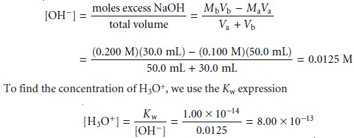
giving a pH of 12.10.
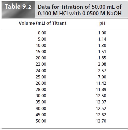
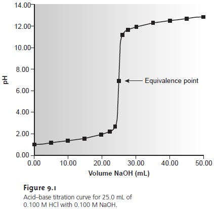
Table 9.2 and Figure 9.1 show additional results for this titra-
tion curve. Calculating the titration curve for the
titration of a strong base
with a strong acid is handled
in the same manner, except
that the strong
base is in excess
before the equivalence point and the strong
acid is in excess after
the equivalence point.
Titrating a Weak Acid with a Strong Base
For this example
let’s consider the titra-
tion of 50.0 mL of 0.100 M acetic acid,
CH3COOH, with 0.100
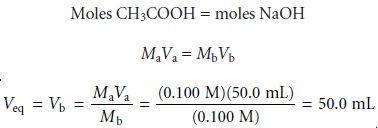
M NaOH. Again,
we start by calculating the volume of NaOH needed
to reach the equivalence point; thus
Before adding any NaOH
the pH is that for
a solution of 0.100 M acetic acid.
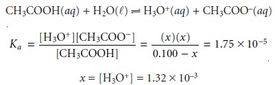
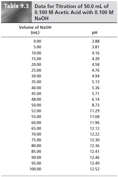
At the beginning of the titration the pH is 2.88.
Adding NaOH converts a portion of the acetic acid to its
conjugate base.

Any
solution containing comparable amounts of a weak acid, HA, and its conjugate weak base, A–, is a buffer.
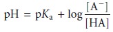
As we learned, we can calculate the pH of a
buffer using the Henderson–Hasselbalch equation.
The
equilibrium constant for
reaction 9.2 is large (K =
Ka/Kw = 1.75 x 10⁹), so we
can treat the reaction as one that goes to completion. Before the equivalence point, the concentration of unreacted acetic
acid is
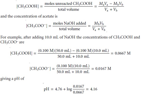
A similar calculation shows that the pH after adding 20.0 mL of
NaOH is 4.58.
At the equivalence point, the moles
of acetic acid initially present
and the moles of
NaOH added are identical. Since
their reaction effectively proceeds to completion, the predominate ion
in solution is CH3COO–, which
is a weak base. To calcu-
late the pH we first
determine the concentration of CH3COO–.

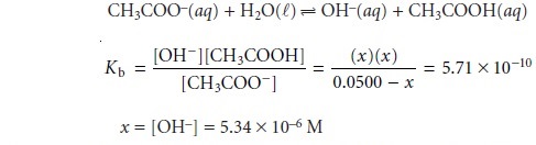
The concentration of H3O+, therefore, is 1.87 x 10⁻⁹, or a pH of
8.73.
After the equivalence point
NaOH is present
in excess, and the pH is deter- mined in the same
manner as in the titration of a strong
acid with a strong base.
For example, after adding
60.0 mL of NaOH, the concentration of OH– is
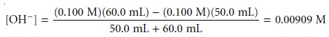
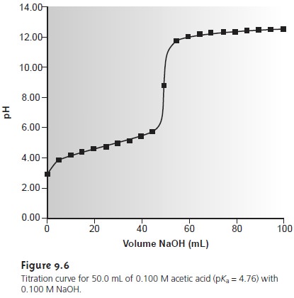
giving a pH of 11.96. Table
9.3 and Figure
9.6 show additional results for this titra-
tion. The calculations for the titration of a weak base with a strong acid are handled
in a similar manner except
that the initial
pH is determined by the weak base,
the pH at the equivalence point by its conjugate weak acid, and the pH after the equiva-
lence point by the concentration of excess strong
acid.
The approach that we have worked out for the titration of a monoprotic weak acid with a strong base can be extended to reactions involving
multiprotic acids or bases
and mixtures of acids or bases. As the complexity of the titration
increases, however, the necessary calculations become more time-consuming.
Not surpris- ingly, a variety
of algebraic1 and computer spreadsheet
approaches have been de-
scribed to aid in constructing titration curves.
Sketching an Acid–Base Titration Curve
To evaluate the
relationship between an equivalence point and an end point,
we only need to construct a reasonable approx- imation to the titration curve. In this section we demonstrate a simple method
for sketching any acid–base titration curve. Our
goal is to sketch the
titration curve quickly, using
as few calculations as possible.
To quickly sketch a titration
curve we take advantage of the following
observa- tion. Except for the initial
pH and the pH at the equivalence point, the pH at any point of a titration curve is determined by either an excess of strong acid
or strong base, or by a buffer consisting of a weak acid and its conjugate weak base. As we
have seen in the preceding sections, calculating the pH of a solution
containing ex- cess strong acid or strong base is straightforward.
We can easily calculate the pH of a buffer using the Henderson–Hasselbalch equa-
tion. We can avoid this calculation, however,
if we make the following assumption. You may
recall that we stated
that a buffer
operates over a pH range ex-
tending approximately ±1 pH units on either
side of the buffer’s pKa. The
pH is at the lower
end of this range, pH = pKa – 1, when the weak acid’s
concentration is approxi- mately ten times greater
than that of its conjugate weak base. Conversely, the buffer’s pH is at its upper limit,
pH = pKa + 1, when the concentration of weak acid is ten times less than that of its conjugate weak base. When titrating a weak acid or weak base, therefore, the buffer
region spans a range of volumes from approximately 10% of the
equivalence point volume to approximately 90% of the equivalence point volume.*
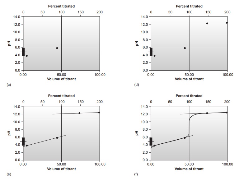
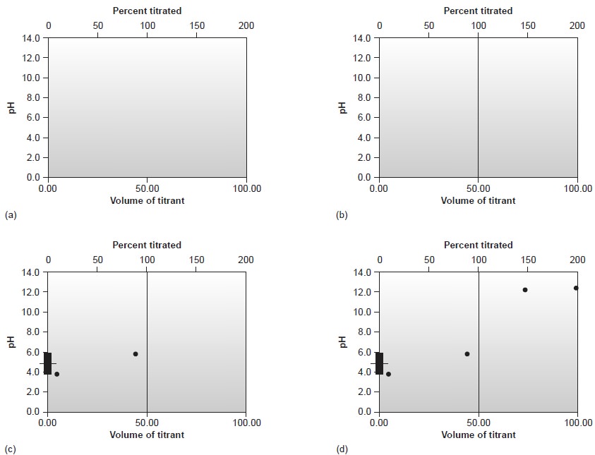
Our strategy
for quickly sketching
a titration curve is simple. We begin by draw- ing our axes, placing
pH on the y-axis and volume of titrant
on the x-axis. After calcu-
lating the volume of titrant
needed to reach the equivalence point, we draw a vertical
line that intersects the x-axis
at this volume.
Next, we determine
the pH for
two vol- umes before
the equivalence point and for two volumes after the equivalence point. To
save time we only calculate pH values
when the pH is determined by excess
strong acid or strong base. For weak acids or bases we use the limits of their buffer region to esti- mate the two points. Straight lines are drawn through
each pair of points,
with each line intersecting the vertical
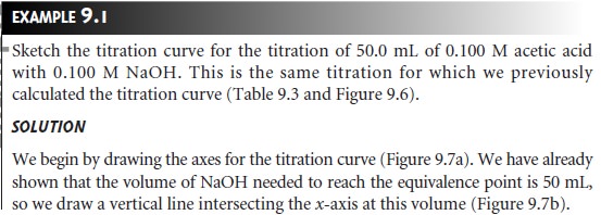
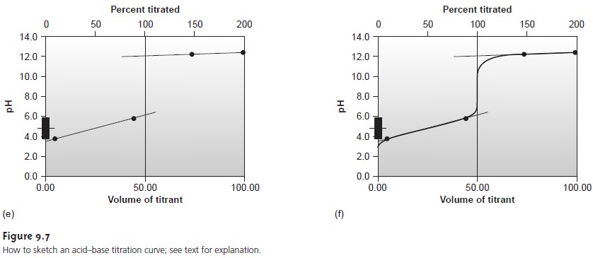
line representing the equivalence point volume. Finally, a smooth curve is drawn connecting the three straight-line segments. Example 9.1 illus- trates this approach for
the titration of a weak acid with a strong base.
This approach can be used to sketch titration curves for other acid–base titra- tions including those involving polyprotic weak acids and bases or mixtures of weak acids and bases (Figure 9.8). Figure 9.8a, for example, shows the titration curve when titrating a diprotic weak acid, H2A, with a strong base.
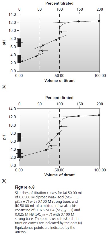
Since the analyte is diprotic
there
are
two
equivalence points, each requiring the same volume of
titrant. Before the first equivalence point the pH is controlled by a buffer consisting
of H2A and
HA–, and
the HA–/A2– buffer determines the pH between the
two equiv- alence points.
After the second
equivalence point, the pH reflects
the concentration of the excess strong
base titrant.
Figure 9.8b shows
a titration curve
for a mixture consisting of two weak acids:
HA and HB. Again, there are two equivalence points.
In this case, however, the equivalence points do not require the same volume
of titrant because
the concen- tration of HA is greater than
that for HB.
Since HA is the stronger of the two
weak acids, it reacts
first; thus, the pH before
the first equivalence point is controlled by the HA/A– buffer. Between the two equivalence points the pH reflects the titration
of HB and is determined by the HB/B– buffer. Finally,
after the second
equivalence point, the excess
strong base titrant
is responsible for
the pH.
Related Topics