Multiple Tasks and Multiple Processes

PROCESSES AND OPERATING SYSTEMS

■The process abstraction.

■Switching contexts between programs. ■Real-time operating systems(RTOSs).

■ Inter process communication.

■Task-level performance analysis and power consumption.

■A telephone answering machine design.

We are particularly interested in real-time operating systems (RTOSs), which are Oss that provide facilities for satisfying real-time requirements. ARTOS allocates resources using algorithms that take real time in to account. General-purpose OSs, incontrast, generally allocate resources using other criteria like fairness. Trying to allocate the CPU equally to all processes with out regard to time can easily cause processes to miss their deadlines. In the next section, we will introduce the concepts of task and process. Introduces some basic concepts in inter process communication. Section6.5con- siders the performance of RTOSs while Section6.6 looks at power consumption. Section 6.7 walks through the design of a telephone answering machine.

MULTIPLE TASKS AND MULTIPLE PROCESSES

Most embedded systems require functionality and timing that is too complex to body in a single program. We break the system in to multiple tasks in order to manage when things happen. In this section we will develop the basic abstractions that will be manipulated by the RTOS to build multirate systems. To understand why these parathion of an application in to tasks may be reflected in the program structure, consider how we would build a stand-alone compression unit based on the compression algorithm we implemented in Section3.7. As shown in Figure6.1, this device is connected to serial ports on both ends. The input to the box is an uncompressed stream of bytes. The box emits a compressed string of bits on the output serial line, based on a predefined compression table. Such a box may be used, for example, to compress data being sent to a modem. The program’s need to receive and send data at different rates—for example, the program may emit 2 bits for the first byte and then 7 bits for the second byte— will obviously find itself reflected in the structure of the code. It is easy to create irregular, ungainly code to solve this problem; a more elegant solution is to create a queue of out put bits, with those bits being removed from the queue and sent to the serial port in 8-bit sets. But beyond the need to create a clean data structure that simplifies the control structure of the code, we must also ensure

that we process the inputs and outputs at the proper rates. For example, if we spend too much time in packaging and emitting output characters, we may drop an input character. Solving timing problems is a more challenging problem.

The text compression box provides a simple example of rate control problems. A control panel on a machine provides an example of a different type of rate con- troll problem, the asynchronous input. The control panel of the compression box may, for example, include a compression mode button that disables or enables com- pression, so that the input text is passed through unchanged when compression is disabled. We certainly do not know when the user will push the compression modebutton— the button may be depressed a synchronously relative to the arrival of characters for compression. We do know, however, that the button will be depressed at a much lower rate than characters will be received, since it is not physically possible for a person to repeatedly depress a button at even slow serial line rates. Keeping up with the input and output data while checking on the button can introduce some very complex control code in to the program. Sampling the button’s state too slowly can cause the machine to miss a button depression entirely, but sampling it too frequently and duplicating a data value can cause the machine to in correctly compress data.

One solution is to introduce a counter in to the main compression loop, so that a subroutine to check the input button is called once every times the compression loop is executed. But this solution does not work when either the compression loop or the button-handling routine has highly variable execution times—if the execution time of either varies significantly, it will cause the other to execute later than expected, possibly causing data to be lost. We need to be able to keep track of these two different tasks separately, applying different timing requirements to each.

This is the sort of control that processes allow. The above two examples illustrate how requirements on timing and execution rate can create major problems in programming. When code is written to satisfy several different timing requirements at once, the control structures necessary to get any sort of solution become very complex very quickly. Worse, such complex control is usually quite difficult to verify for either functional or timing properties.

Multi rate Systems

Implementing code that satisfies timing requirements is even more complex when multiple rates of computation must be handled. Multi rate embedded computing systems are very common, including auto mobile engines, printers, and cell phones.In all these systems, certain operations must be executed periodically, and each oper-ation is executed at its own rate. Application Example6.1 describes why auto mobile engines require multi rate control.

Timing Requirements on Processes

Processes can have several different types of timing requirements imposed on them by the application. The timing requirements on a set of process strongly influence the type of scheduling that is appropriate. A scheduling policy must define the timing requirements that it uses to determine whether a schedule is valid. Before studying scheduling proper, we outline the types of process timing requirements that are useful in embedded system design. Figureillustrates different ways in which we can define two important requirements on processes: eg. What happens when a process misses a deadline? The practical effects of a timing violation depend on the application—the results can be catastrophic in an auto mo- tive control system, where as a missed deadline in a multi media system may cause an audio or video glitch. The system can be designed to take a variety of actions when a deadline is missed. Safety-critical systems may try to take compensatory measures such as approximating data or switching in to a special safety mode. Systems for which safety is not as important may take simple measures to avoid propagating bad data, such as inserting silence in a phone line, or may completely ignore the failure.Even if the modules are functionally correct, their timing improper behavior can introduce major execution errors. Application Example6.2 describes a timing problem in space shuttle software that caused the delay of the first launch of the shuttle. We need a basic measure of the efficiency with which we use the CPU. The simplest and most direct measure is utilization:

Utilization is the ratio of the CPU time that is being used for useful computations to the total available CPUtime. This ratio ranges between 0 and 1, with 1 meaning that all of the available CPU time is being used for system purposes. The utilization is often expressed as a percentage. If we measure the total execution time of all processes over an interval of time t, then the CPU utilization is U/T

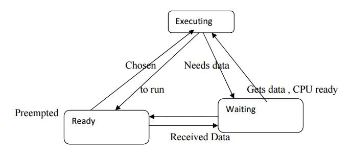
Process State and Scheduling

The first job of the OS is to determine that process runs next. The work of choosing the order of running processes is known as scheduling. The OS considers a process to be in one of three basic scheduling states

Schedulability means whether there exists a schedule of execution for the processes in a system that satisfies all their timing requirements. In general, we must construct a schedule to show schedulability, but in some cases we can eliminate some sets of processes as unschedulable using some very simple tests. Utilization is one of the key metrics in evaluating a scheduling policy. Our most basic require- ment is that CPU utilization be no more than 100% since we can’t use the CPU more than100% of the time.

When we evaluate the utilization of the CPU, we generally do so over a finite period that covers all possible combinations of process executions. For periodic processes, the length of time that must be considered is the hyper period, which is the least-common multiple of the periods of all the processes. If we evaluate the hyper period, we are sure to have considered all possible combinations of the periodic processes. The next example evaluates the utilization of a simple set of processes.

We will see that some types of timing requirements for a set of processes imply that we can not utilize 100% of the CPU’s execution time on useful work, even ignoring context switching overhead. However, some scheduling policies can deliver higher CPU utilizations than others, even for the same timing requirements. The best policy depends on the required timing characteristics of the processes being scheduled.

On every simple scheduling policy is known as cyclostatic scheduling or some- times as Time Division Multiple Access scheduling. Processes always run in the same time slot. Two factors affect utilization: the number of times lots used and the fraction of each time slot that is used for useful work. Depending on the deadlines for some of the processes, we may need to leave some times lots empty. And since the time slots are of equal size, some short processes may have time left over in their time slot. We can use utilization as a schedulability measure: the total CPU time of all the processes does not have any useful work to do, the round-robin scheduler moves on to the next process in order to fill the time slot with useful work. In this example, all three processes execute during the first hyper period, but during the second one, P1 has no useful work and is skipped. The processes are always evaluated in the same order. The last time slot in the hyper period is left empty; if we have occasional, non-periodic tasks with out deadlines, we can execute them in these empty time slots. Round-robin scheduling is often used in hardware such as buses because it is

Very simple to implement but it provides some amount of flexibility. In addition to utilization, we must also consider scheduling overhead—the execution time required to choose the next execution process, which is incurred in addition to any context switch in gover head. In general, the more sophisticated the scheduling policy, the more CPU time it takes during system operation to implement it. Moreover, we generally achieve higher theoretical CPU utilization by applying more complex scheduling policies with higher over heads. The final decision on a scheduling policy must take in to account both theoretical utilization and practical scheduling overhead.

Running Periodic Processes

We need to find a programming technique that allows us to run periodic processes, ideally at different rates. For the moment, let’s think of a process as a subroutine; we will call the mp1(), p2(), etc. for simplicity. Our goal is to run these subroutines at rates determined by the system

designer. Here is a very simple program that runs our process subroutines repeatedly: A timer is a much more reliable way to control execution of the loop. We would probably use the timer to generate periodic interrupts. Let’s assume for the moment that the pall() function is called by the timer’s interrupt handler. Then this code will execute each process once after a timer interrupt:

voidpall() {

p1();

p2();

}

But what happens when a process runs too long? The timer’s interrupt will cause the CPU’s interrupt system to mask its interrupts, so the interrupt will not occur until after the pall() routine returns. As a result, the next iteration will start late. This is a serious problem, but we will have to wait for further refinements before we can fix it.

Our next problem is to execute different processes at different rates. If we have several timers, we can set each timer to a different rate. We could then use a function to collect all the processes that run at that rate:

voidpA() {

/*processesthatrunatrateA*/

p1();

p3();

}

voidpB() {

/*processesthatrunatrateB*/

This solution allows us to execute processes at rates that are simple multiples of each other. However, when the rates are n’t related by a simple ratio, the counting process becomes more complex and more likely to contain bugs. We have developed some what more reliable code, but this programming style is still limited in capability and prone to bugs. To improve both the capabilities and reliability of our systems, we need to invent the RTOS.