Chapter: Modern Analytical Chemistry: Spectroscopic Methods of Analysis
Absorbance and Concentration: Beer’s Law
Absorbance and Concentration: Beer’s Law
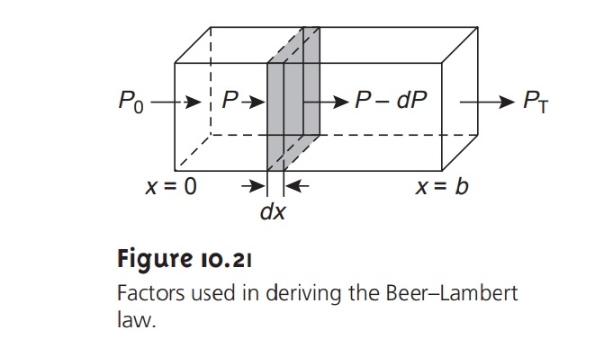
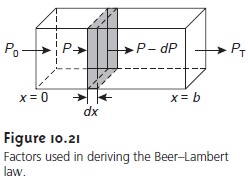
When monochromatic electromagnetic radiation passes through
an infinitesimally thin layer
of sample, of thickness dx, it
experiences a decrease
in power of dP (Figure 10.21). The fractional decrease
in power is proportional to the sample’s
thick- ness and the
analyte’s concentration, C; thus
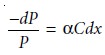 10.3
10.3
where P is the power incident
on the thin layer of sample, and α is a proportionality constant. Integrating the left side of equation
10.3 from P =
P0 to P = PT, and the
right side from x = 0 to x =
b, where b is the
sample’s overall thickness
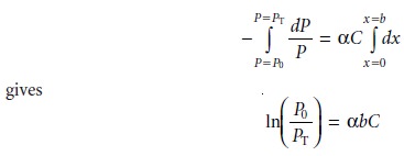
Converting from ln to log, and substituting equation 10.2, gives
A =
abC …………. 10.4
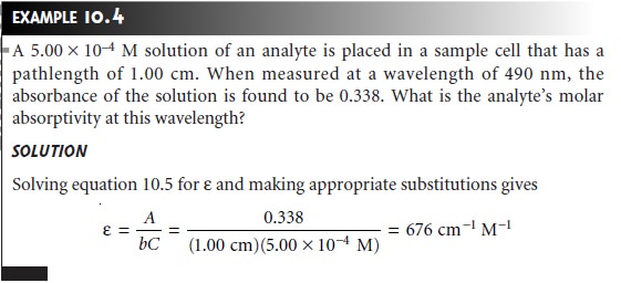
where a is the analyte’s absorptivity with units of cm–1 conc–1. When concentration is expressed using molarity, the absorptivity is replaced by the molar
absorptivity, ε (with units
of cm–1
M–1)
A =
εbC …………. 10.5
The absorptivity and molar absorptivity give, in effect,
the probability that the ana- lyte
will absorb a photon of given energy.
As a result, values for both a and
ε depend on the
wavelength of electromagnetic radiation.
Equations 10.4 and 10.5, which establish the linear relationship
between absorbance and concentration, are known as the Beer–Lambert law, or more commonly, as Beer’s law. Calibration curves
based on Beer’s
law are used routinely in quantitative
analysis.
Beer’s Law and Multicomponent Samples
Beer’s law can be extended to samples containing several
absorbing components provided that there
are no interactions between the components. Individual ab-
sorbances, Ai, are additive. For a two-component mixture of X and Y, the total
ab- sorbance, Atot, is
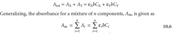
Related Topics