Chapter: Modern Analytical Chemistry: Equilibrium Chemistry
Ladder Diagrams
Ladder Diagrams
When developing or evaluating an analytical method,
we often need to under- stand how
the chemistry taking
place affects our
results. We have
already seen, for example,
that adding NH3 to a solution
of Ag+ is a poor idea if we intend to isolate the Ag+ as a precipitate of AgCl (reaction 6.29). One of the primary
sources of determinate method errors is a failure
to account for potential chemi-
cal interferences.
In this section
we introduce the ladder diagram as
a simple graphical tool for evaluating the chemistry taking
place during an analysis.
Using ladder dia- grams, we will be able to determine what reactions occur
when several reagents are combined, estimate the
approximate composition of a system
at equilibrium, and evaluate how a change
in solution conditions might affect our results.
Ladder Diagrams for Acid–Base Equilibria
To see how a ladder
diagram is constructed, we will use the acid–base equilibrium between HF and F–

Finally, replacing the negative log terms with p-functions and rearranging leaves
us with
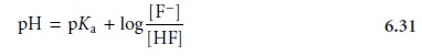
Examining equation 6.31 tells us a great deal about the relationship
between pH and the
relative amounts of F– and HF at equilibrium. If the concentrations of F– and HF are equal,
then equation 6.31 reduces to
pH=
pKa,HF = –log(Ka,HF) = –log(6.8 x 10⁻⁴) = 3.17
For concentrations of F– greater than that of HF, the
log term in equation 6.31
is positive and
pH>
pKa,HF or pH
> 3.17
This is a reasonable result since we expect the concentration of hydrofluoric acid’s conjugate base, F–, to increase as the pH increases. Similar
reasoning shows that the
concentration of HF exceeds that
of F–
when
pH < pKa,HF
or pH < 3.17
Now
we
are
ready
to
construct the ladder diagram for HF (Figure 6.4).
The
ladder
diagram
consists
of
a vertical
scale of pH values oriented so that smaller
(more acidic) pH levels are at the bottom and larger (more basic) pH levels
are at the top. A horizontal line is drawn
at a pH equal to pKa,HF. This line, or step,
separates the solution
into regions where
each of the two conjugate forms of HF predominate.
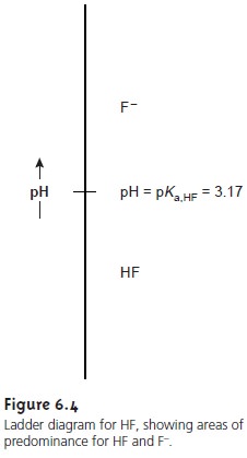
By
referring to the ladder diagram, we see that at a pH of 2.5 hydrofluoric acid will exist
predominately as HF. If we add sufficient base to the solution
such that the pH increases to 4.5, the
predominate form be- comes F–.
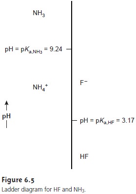
Figure 6.5 shows a second ladder diagram containing information
about HF/F– and NH4 +/NH3 . From
this ladder diagram
we see that if the pH is less
than 3.17, the predominate species
are HF and
NH4+. For
pH’s between 3.17 and 9.24 the predominate species are F– and NH4+, whereas above a pH of 9.24
the predominate species are F– and NH3.
Ladder diagrams are
particularly useful for
evaluating the reactivity of acids and bases.
An acid and a base cannot coexist
if their respective areas of
predominance do not overlap. If we mix together solutions of NH3 and HF,
the reaction

occurs because
the predominance areas
for HF and NH3 do not overlap.
Be- fore continuing, let us show that this conclusion is reasonable by calculating
the equilibrium constant
for reaction 6.32.
To do so we need the following three reactions and their
equilibrium constants.

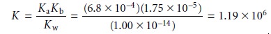
Since the equilibrium constant is significantly greater than 1, the reaction’s equilib- rium position lies far to the right.
This conclusion is general and applies to all lad- der
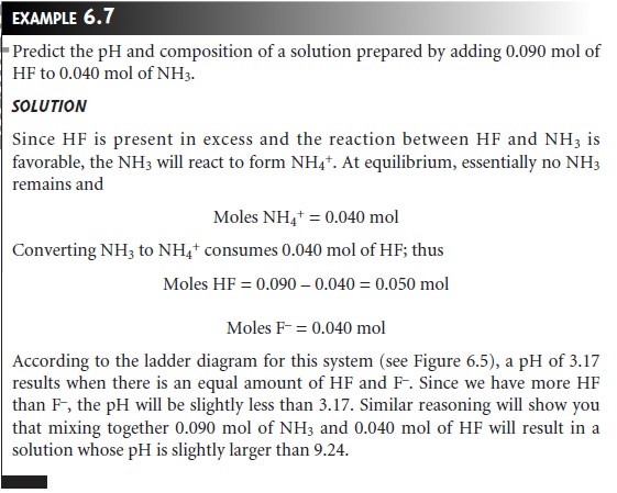
diagrams. The following example shows how we can use the ladder diagram
in Figure 6.5 to evaluate the composition of any solution
prepared by mixing together
solutions of HF and NH3.
If the areas
of predominance for an acid and a base overlap
each other, then practically no reaction occurs.
For example, if we mix together solutions
of NaF and NH4Cl, we expect that there will be no significant change in the moles of F– and NH4+. Furthermore, the pH of the mixture
must be between
3.17 and 9.24.
Because F– and NH4+ can coexist over a range of pHs we cannot be more specific in estimat- ing the solution’s pH.
The
ladder
diagram
for
HF/F– also can be used to evaluate the effect of
pH on other
equilibria that include
either HF or F–. For
example, the solubility of CaF2
CaF2(s) < = = = > tCa2+(aq)+ 2F–(aq)
is affected by pH because
F– is a weak base.
Using Le Châtelier’s principle, if F– is
converted to HF, the solubility of CaF2 will
increase. To minimize the solubility of CaF2 we want to control the solution’s pH so that F– is the predominate species. From the ladder diagram
we see that maintaining a pH of more than 3.17 ensures that solubility losses are minimal.
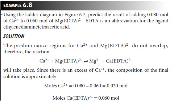
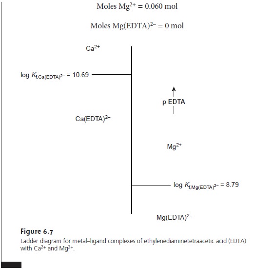
Ladder Diagrams for Complexation Equilibria
The same principles used in constructing and interpreting ladder
diagrams for acid–base equilibria can be applied to equilibria
involving metal–ligand com- plexes. For complexation reactions
the ladder diagram’s
scale is defined
by the concentration of uncomplexed, or free ligand, pL. Using the formation of Cd(NH3)2+ as an example
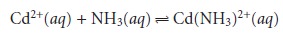
we can easily show that the dividing line between the
predominance regions for Cd2+ and Cd(NH3)2+ is log(K1).
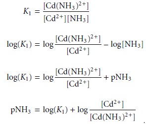
Since K1 for Cd(NH3)2+ is 3.55 ´ 102,
log(K1) is 2.55. Thus, for a pNH3 greater than 2.55
(concentrations of NH3 less than 2.8 x 10⁻³ M), Cd2+
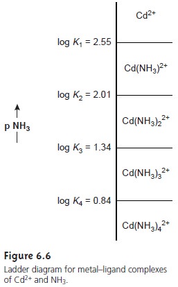
is the predominate species. A complete ladder diagram for the metal–ligand
complexes of Cd2+ and NH3 is shown in Figure 6.6.
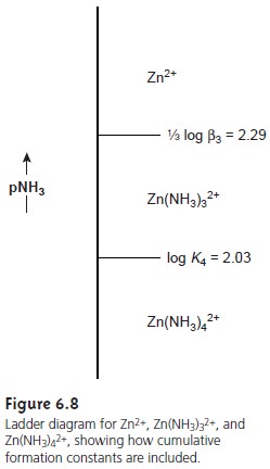
We can also construct ladder
diagrams using cumulative formation constants
in place of stepwise formation constants. The first
three stepwise formation con- stants for the reaction of Zn2+ with NH3
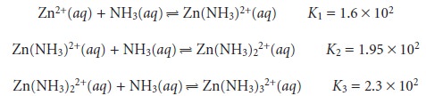
show that the formation of Zn(NH3)32+ is more favorable than the formation of Zn(NH3)2+ or Zn(NH3)22+. The equilibrium, therefore, is best represented by the cumulative
formation reaction
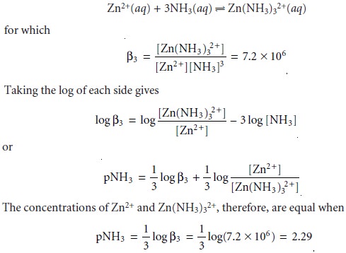
A complete ladder
diagram for the Zn2+–NH3 system
is shown in Figure 6.8.
Ladder Diagram for Oxidation–Reduction Equilibria
Ladder diagrams can
also be used
to evaluate equilibrium reactions in redox
sys- tems. Figure 6.9 shows a typical ladder
diagram for two half-reactions in which
the scale is the electrochemical potential, E. Areas of predominance are defined by the
Nernst equation. Using
the Fe3+/Fe2+
half-reaction as an example, we write
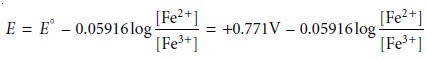
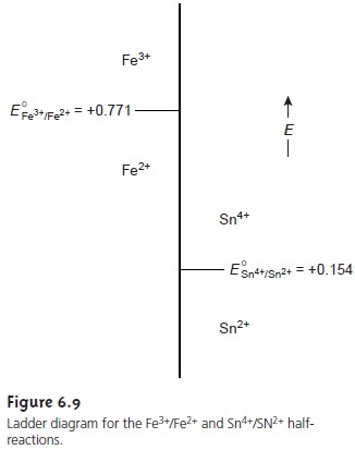
For potentials more positive than the standard-state potential, the predominate species is Fe3+, whereas
Fe2+ predominates for potentials more negative than E°. When coupled with the step for the Sn4+/Sn2+ half-reaction, we see that Sn2+ can be used to reduce
Fe3+. If an excess
of Sn2+
is added, the potential of the resulting solu- tion will be near +0.154 V.
Using standard-state potentials to construct a ladder diagram
can present problems if solutes are not at their standard-state concentra- tions. Because the concentrations of the reduced
and oxidized species are in a logarithmic term,
deviations from standard-state concentra-
tions can usually be ignored
if the steps being compared
are separated by at least 0.3 V.1b A
trickier problem occurs
when a half-reaction’s po-
tential is affected by the concentration of another species.
For example, the potential for the following half-reaction

depends on the
pH of the solution. To define areas
of predominance in this
case, we begin
with the Nernst
equation
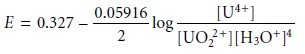
and factor out the concentration of H3O+.
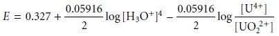
From this equation we see that the areas of predominance for UO22+ and U4+ are defined
by a step whose potential is
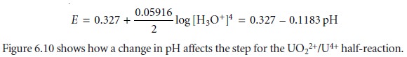
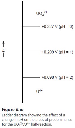
Related Topics