Buffer Solutions

Buffer Solutions

Adding as little as 0.1 mL of concentrated HCl to a liter of H₂O shifts the pH from 7.0 to 3.0. The same addition of HCl to a liter solution that is 0.1 M in both a weak acid and its conjugate weak base, however, results in only a negligible change in pH. Such solutions are called buffers, and their buffering action is a consequence of the relationship between pH and the relative concentrations of the conjugate weak acid/weak base pair.

A mixture of acetic acid and sodium acetate is one example of an acid/base buffer. The equilibrium position of the buffer is governed by the reaction

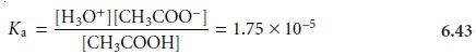
CH₃COOH(aq)+ H₂O(l)  < == == >  H₃O+(aq)+ CH₃COO–(aq)

and its acid dissociation constant

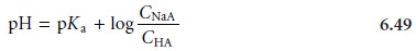
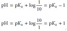
The relationship between the pH of an acid–base buffer and the relative amounts of CH₃COOH and CH₃COO– is derived by taking the negative log of both sides of equation 6.43 and solving for the pH

Buffering occurs because of the logarithmic relationship between pH and the ratio of the weak base and weak acid concentrations. For example, if the equilibrium concentrations of CH₃COOH and CH₃COO– are equal, the pH of the buffer is 4.76. If sufficient strong acid is added such that 10% of the acetate ion is converted to acetic acid, the concentration ratio [CH₃COO–]/[CH₃COOH] changes to 0.818, and the pH decreases to 4.67.

Systematic Solution to Buffer Problems

Equation 6.44 is written in terms of the concentrations of CH₃COOH and CH₃COO– at equilibrium. A more useful relationship relates the buffer’s pH to the initial concentrations of weak acid and weak base. A general buffer equation can be derived by considering the following reactions for a weak acid, HA, and the salt of its conjugate weak base, NaA.

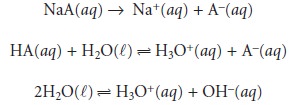
Since the concentrations of Na+, A–, HA, H₃O+, and OH– are unknown, five equa- tions are needed to uniquely define the solution’s composition. Two of these equa- tions are given by the equilibrium constant expressions

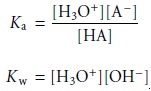
The remaining three equations are given by mass balance equations on HA and Na+

C_HA + C_NaA = [HA]+ [A–]              6.45

C_NaA = [Na+]              6.46

and a charge balance equation

[H₃O+] + [Na+] = [OH–]+ [A–]

Substituting equation 6.46 into the charge balance equation and solving for [A–] gives

[A–]= C_NaA – [OH–]+ [H₃O+]              6.47                                  

which is substituted into equation 6.45 to give the concentration of HA

[HA] = C_HA + [OH–]– [H₃O+]              6.48                                   

Finally, substituting equations 6.47 and 6.48 into the K_a equation for HA and solv- ing for pH gives the general buffer equation

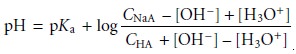
If the initial concentrations of weak acid and weak base are greater than [H₃O+] and [OH–], the general equation simplifies to the Henderson–Hasselbalch equation.

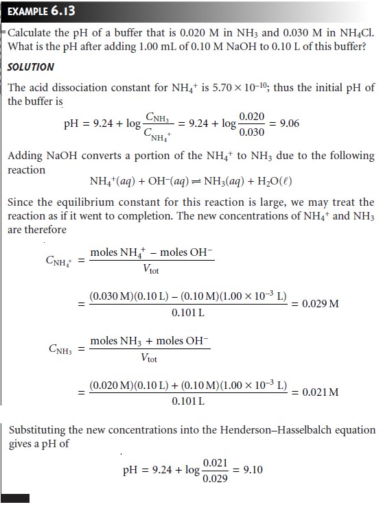
As in Example 6.13, the Henderson–Hasselbalch equation provides a simple way to

calculate the pH of a buffer and to determine the change in pH upon adding a strong acid or strong base.

Multiprotic weak acids can be used to prepare buffers at as many different pH’s as there are acidic protons. For example, a diprotic weak acid can be used to prepare buffers at two pH’s and a triprotic weak acid can be used to prepare three different buffers. The Henderson–Hasselbalch equation applies in each case. Thus, buffers of malonic acid (pK_a1 = 2.85 and pK_a2 = 5.70) can be prepared for which

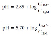
where H₂M, HM–, and M2– are the different forms of malonic acid.

The capacity of a buffer to resist a change in pH is a function of the absolute concentration of the weak acid and the weak base, as well as their relative propor- tions. The importance of the weak acid’s concentration and the weak base’s con- centration is obvious. The more moles of weak acid and weak base that a buffer has, the more strong base or strong acid it can neutralize without significantly changing the buffer’s pH. The relative proportions of weak acid and weak base af- fect the magnitude of the change in pH when adding a strong acid or strong base. Buffers that are equimolar in weak acid and weak base require a greater amount of strong acid or strong base to effect a change in pH of one unit. Consequently, buffers are most effective to the addition of either acid or base at pH values near the pK_a of the weak acid.

Buffer solutions are often prepared using standard “recipes” found in the chemical literature. In addition, computer programs have been developed to aid in the preparation of other buffers. Perhaps the simplest means of preparing a buffer, however, is to prepare a solution containing an appropriate conjugate weak acid and weak base and measure its pH. The pH is easily adjusted to the desired pH by adding small portions of either a strong acid or a strong base.

Although this treatment of buffers was based on acid–base chemistry, the idea of a buffer is general and can be extended to equilibria involving complexation or redox reactions. For example, the Nernst equation for a solution containing Fe2+ and Fe3+ is similar in form to the Henderson–Hasselbalch equation.

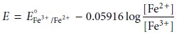
Consequently, solutions of Fe2+ and Fe3+ are buffered to a potential near the standard-state reduction potential for Fe3+.

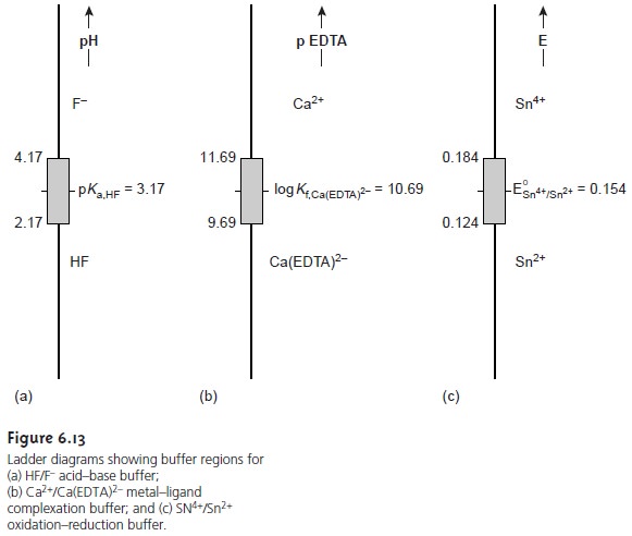
Representing Buffer Solutions with Ladder Diagrams

Ladder diagrams provide a simple graphical description of a solution’s predominate species as a function of solution conditions. They also provide a convenient way to show the range of solution conditions over which a buffer is most effective. 

For example, an acid–base buffer can only exist when the relative abundance of the weak acid and its conjugate weak base are similar. For convenience, we will assume that an acid–base buffer exists when the concentration ratio of weak base to weak acid is between 0.1 and 10. Applying the Henderson–Hasselbalch equation

shows that acid–base buffer exists within the range of pH = pK_a ± 1. In the same manner, it is easy to show that a complexation buffer for the metal–ligand complex ML_n exists when pL = log K_f ± 1, and that a redox buffer exists for E = E° ± (0.05916/n). Ladder diagrams showing buffer regions for several equilibria are shown in Figure 6.13.