Modal response contribution using Chopra’s method

Modal response contribution using Chopra’s method (Chopra, 2002)

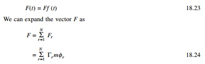
The forced vibration of undamped system and the dynamic equation of motion may be written as

mu˙˙ + ku = F (t )                 --- --- 18.22

We now consider the common loading case in which the force F_j(t) have the same time variation f (t) and their spatial distribution is defined, independent of time. Thus

where φ_r is the normalized eigenvector for the rth mode.

Pre-multiplying both sides with φ_n^T and utilizing the orthogonalization property of the modes we get

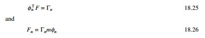
which is independent of how the modes are normalized.

Equation 18.26 may be viewed as an expression of the distribution F of applied force in terms of force distribution F_n associated with natural period. This interpretation becomes apparently clear by considering the structure vibration in the n th mode with acceleration u˙˙_n = φ_n ˙˙y_n ( t ) . The associated inertia force = − mu˙˙_n (t ) = − mφ_n ˙˙y_n and their spatial distribution given by vector mφ_n which is same as F_n.

Two useful properties are to be noted:

1.     The force vector F_n f (t) produces response only in the nth mode, there is no response in another mode.

2.     This dynamic response in the nth mode is entirely due to the partial force vector F_np(t).

Example 18.4

Consider a five storey building (rigid floor beams and slabs) with lumped mass m at each floor, and same storeyed stiffness k. <F>= <0 0 –1 1 2). See Fig. 18.8.

Solution

Use the MATHEMATICA or MATLAB package. Assume k = 1 m = 1.

Using the MATLAB program we get five natural frequencies and five normalized mode shapes.

ω₁ = 0.2439; ω₂ = 0.6689; ω₃ = 1.0; ω₄ = 1.286; ω₅ = 1.6850 rad/s

Modal analysis for Γ f (t)

The factor Γ_n which multiplies the force f (t) is sometimes known as the modal participation factor, implying that it is a measure of the degree to which the nth mode participates in the response. This is not a useful definition because Γ_n is not independent of how the mode is normalized or a measure of the contribution of the mode to a response quantity. Both these drawbacks are overcome by the modal contribution factor.

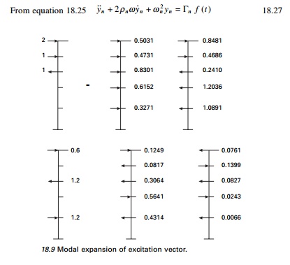
Let us consider the uncoupled equation of motion

Hence y_n is readily available once equation 18.30 has been solved for D_n (t) utilizing the available result of single-degree-of-freedom (SDOF) systems say, for example, subjected to harmonic step impulsive forces, etc.

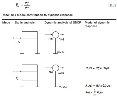
which is the contribution of the nth mode of modal displacement u(t). Substituting Eq. 18.30 to get the equivalent static force as

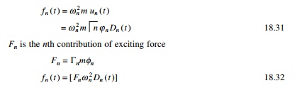
The nth mode contribution to any response quantity R(t) is determined by static analysis of structures subjected to forces f_n(t). If R_n^st denotes the modal static response, the static value indicating ‘st’ of R due to external force F_n then

The model analysis procedure just presented is a special case of the one presented earlier. It has the advantage of providing a basis for identifying and understanding the factors that influence the relative modal contributions to the response. The above procedure can be applied only if the f (t) for all the forces are the same.

Interpretation of modal analysis

1.     Determine natural frequencies and modes.

2.     Force distribution is expanded into modal components {F}.

The rest of the procedure is explained in Table 18.1.

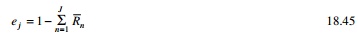
Modal contribution factor

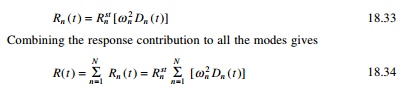
The contribution R_n of the nth mode to response quantity R can be expressed

where R^st is the static value of R due to external force F and the nth modal contribution factor is defined as

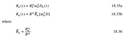
These modal contribution factors have three important properties:

1.     They are dimensionless.

2.     They are independent of how modes are normalized.

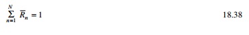
3.     The sum of modal contribution factors over all modes is unity.

Modal response and required number of modes

Consider the displacement D_n(t) of the nth mode SDOF system. The peak value is defined as

D_n0 = Max _t| D_n(t) |               --- ---18.39a

The corresponding value R_n(t) is

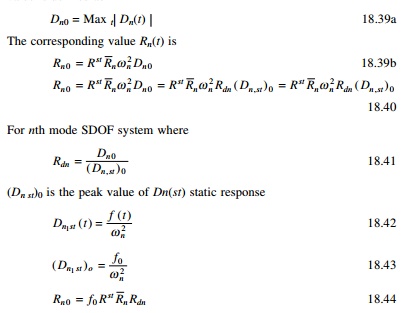
The algebraic system of R_no is same as the modal static response R_n^st = R ^st R_n . The modal contribution factor dynamic response factor R(t) influences the relative response contribution of vibration mode, and hence the minimum number of modes that should be included in dynamic analysis. If only J modes are included in the static response

For a fixed J, e_j depends on spatial distribution of F of the applied force. When all modes are included e_j = 0. Hence modal analysis can truncate modes when | e_j | < ε. Hence most important factors are modal contribution factor and dynamic response factors.

Modal contributions

For the five storey situation three modes are required for base shear and two modes are required for roof displacement.

Example 18.5

For the five storey building example

F(t) = Ff (t); < F >=< 0 0 – 1 1 2>

The system is undamped. Compute only the steady state response.

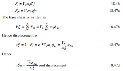
Example 18.6

Figure 18.11 shows a shear frame (i.e. rigid beams) and its floor masses and storey stiffness. This structure is subjected to horizontal harmonic force at the top floor. p₀ = 500 kN.

(a)  Determine the equation for steady state displacement of the structure.

(b) Determine the direct solution of coupled equations.

(c)  Determine the modal analysis (neglect damping).

(d) If k = 63 600 kN/m, m = 45 413 kg and ω = 0.75 ω₁ split the load into modal components and obtain the solution using Chopra’s method.

Solution

Example 18.7

Figure 18.13 shows a mass-less simply suported beam with three lumped masses and the following properties: L = 3.81 m, m = 33 665 kg, E = 207.15 GPa.

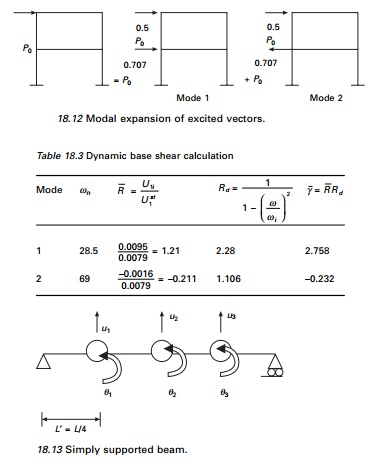
We are interested in studying the dynamic response of the beam to F(t) = Ff(t) where < F >=<1 0 0>.

(a)  Determine the modal expansion of vector {F} that defines the spatial distribution of force.

(b)For the bending moment M₁ at the location of U₁ degrees of freedom determine the modal static response

(c)  Calculate and tabulate modal contribution factors their cumulative values for various numbers of modes included J = 1, 2, 3 and the error e_j for static response. Comment on how the relative values of modal contribution factors and the error e_j are influenced by spatial distribution of forces.

(d)Determine the peak value of (M_1n)₀ modal response due to F(t)

Assume t_d = 0.598 s which is the same as T₁.

The distribution of the pulse td = T₁ the fundamental period of the system. For the shock spectrum of half cycle sine wave R_d = 1.73, 1.14 and 1.06 for T₁/t_d = 1; T₂/t_d = 0.252; T₃/t_d = 0.119 respectively. It will be convenient to organize the computation in a table with following headings: n, T_n/t_d, R_dn, M_1n and [( M_{1 n} )₀ /( p ₀ M₁^st )]

(e)  Comment on how the peak modal response determined in part (d) depend on modal static response, modal contributed factor M_1n and R_dn and S.

(f)   Is it possible to determine the peak value of the total (considering all modes) response from peak modal response? Justify your answer.

E = 207.15 GPa m = 33 665 kg

L = 3.81 m

I = 4.1623 × 10⁷ mm⁴

Step 7 Determine modal static response as shown in Fig. 18.16. The value of moments due to forces F is determined by the linear combination to the above three load cases. The resultants are as given in Table 18.5.

Next we can determine

Step 8 Determine modal contribution factors, their cumulative values and error.

The modal contribution factors and error are given in Table 18.6

In the above the modal contribution factor is largest for first mode and progressively decreases for the second and third modes.

Step 9 Determine response to the half cycle sine pulse. The peak modal response equation is specialized for R = M₁ to obtain (see Table 18.7)

Step 10 Comments

•       For the given force, the modal response decreases for higher modes. The decrease is more rapid because of R_dn. It also decreases with mode n.

The peak value of the total response cannot be determined from the peak modal response because the modal peaks occur at different time instants. Square root of sum of squares (SRSS) and complete quadratic combination (CQC) do not apply to pulse excitations.

Program 18.1: MATLAB program to find the ratio of dynamic shear to static shear in a multi-storey building

%program to get modal components of the forces and calculate

%ratio of dynamic shear to static shear

clc; close all;

% m=45413*[1 0;0 0.5];

m=[1 0 0 0 0;0 1 0 0 0;0 0 1 0 0;0 0 0 1 0;0 0 0 0 1]; disp(‘ mass matrix’)

m

%you can give stiffness matrix disp(‘ stiffness matrix’)

% k=63600000*[2 -1 ;-1 1];

k=[2 -1 0 0 0;-1 2 -1 0 0;0 -1 2 -1 0;0 0 -1 2 -1;0 0 0 -1 1]; k

a=inv(k);

%or you can given flexibility matrix directly

%a=[.75 .5 .25;.5 1 .5;.25 .5 .75];

disp(‘ flexibility matrix’) a

c=a*m;

[ms,ns]=size(m);

par=zeros(ns,ns);

%force vector

%s=[0;500000] s=[0;0;0;-1;2]; su=0;

for i=1:ns su=su+s(i);

end

%imposed frequency

%omimp=21.376;

disp(‘ imposed frequency’) omimp=0.15

%eigen values and eigen vectors [V,D]=eig(c);

for i=1:ms e(i)=1/D(i,i);

end Qh=max(e)+0.001; Ql=0;

for i=1:ms for j=1:ms

if e(j) > Ql & e(j) < Qh kk=j;

Qh=e(j); else

end end Ql=Qh;

Qh=max(e)+0.001;

om1(i)=e(kk);

omega(i)=sqrt(e(kk)); for l=1:ms

p1(l,i)=V(l,kk); end

end

%Normalizing the mode shape L=p1'*m*p1;

%develop modal matrix for i=1:ms

for j=1:ms p(i,j)=p1(i,j)/sqrt(L(j,j));

end end

disp(‘ Natural frequencies in rad/sec’) disp(omega)

disp(‘ normalized modal vector’) disp(p)

disp(‘ check pT m p=I’) p’*m*p

%for earthquake analysis %s=[m(1,1);m(2,2);m(3,3);m(4,4);m(5,5)] gamma=p’*s;

for i=1:ns par(i,i)=gamma(i);

end

%modal contribution of forces

disp(‘ modal contribution of forces’) ee=m*p*par

disp(‘ dynamic magnification factors’) for i=1:ns

rdn(i,i)=1/(1-(omimp/omega(i))^2); end

rdn ust=a*ee; u=ust*rdn; for i=1:ns

dis(i)=0; for j=1:ns

dis(i)=dis(i)+u(i,j); end

end

%disp(‘ amplitude of displacements’); dis;

fo=k*dis’;

sum=0; for i=1:ns

sum=sum+fo(i); end

ratio=sum/su;

disp(‘ ratio of dynamic base shear to static shear’) ratio

OUTPUT mass matrix

a =                                

1.0000        1.0000        1.0000        1.0000        1.0000

1.0000        2.0000        2.0000        2.0000        2.0000

1.0000        2.0000        3.0000        3.0000        3.0000

1.0000        2.0000        3.0000        4.0000        4.0000

1.0000        2.0000        3.0000        4.0000        5.0000

imposed frequency

omimp =                                 

0.1500                                    

Natural frequencies in rad/sec          

0.2846        0.8308        1.3097        1.6825        1.9190

normalized modal vector                           

–0.1699      –0.4557      –0.5969      –0.5485      0.3260

–0.3260      –0.5969      –0.1699      0.4557        –0.5485

–0.4557      –0.3260      0.5485        0.1699        0.5969

–0.5485      0.1699        0.3260        –0.5969      –0.4557

–0.5969      0.5485        –0.4557      0.3260        0.1699

check pT m p=I

ans =                             

1.0000        –0.0000      –0.0000      –0.0000      0.0000

–0.0000      1.0000        0.0000        0.0000        0.0000

–0.0000      0.0000        1.0000        0.0000        –0.0000

–0.0000      0.0000        0.0000        1.0000        –0.0000

0.0000        0.0000        –0.0000      –0.0000      1.0000

modal contribution of forces

ee =

0.1096        –0.4225      0.7386        –0.6851      0.2594

0.2104        –0.5534      0.2102        0.5692        –0.4364

0.2941        –0.3023      –0.6788      0.2122        0.4748

0.3539        0.1575        –0.4034      –0.7455      –0.3625

0.3851        0.5086        0.5640        0.4072        0.1352

dynamic magnification factors

rdn =                             

1.3845        0        0        0        0

0        1.0337        0        0        0

0        0        1.0133        0        0

0        0        0        1.0080        0

0        0        0        0        1.0061

ratio of dynamic base shear to static shear

ratio =

1.5039