Chapter: Civil : Structural dynamics of earthquake engineering
Free vibration of multiple degrees of freedom
Free vibration of multiple degrees of freedom in relation to structural dynamics during earthquakes
Abstract: In this chapter, free and forced vibration of the multiple-degrees-of-freedom (MDOF) system are discussed. The generalized equations are obtained by applying either NewtonŌĆÖs second law or solving Lagrange equations. The orthogonality principle between modes is illustrated. It is also shown how modes are normalized. The stiffness method is used to derive the stiffness matrix of a structure. Relevant programs in MATHEMATICA and MATLAB are also given.
Key words: CordonŌĆÖs solution, orthogonality, normalization, stiffness method, static condensation.
Introduction
After having seen the behaviour of two degrees of freedom, we now proceed to a more general treatment of the problem. Analysis of two degrees of freedom is more involved than a single degree of freedom. When more masses are considered, the mathematical formulation becomes much more complicated. Most engineering systems are continuous and have an infinite number of degrees of freedom. The vibration analysis of continuous systems requires the solution of partial differential equations which is quite difficult. In fact a solution is not available for many partial differential equations. The analysis of multiple degrees of freedom (MDOF), on the other hand, requires the solution of a set of ordinary differential equation which is relatively simple. Hence, for simplicity of analysis, continuous systems are often approximated as MDOF. All the concepts introduced in the previous chapters can be directly extended to the case of MDOF. One can write one differential equation of equilibrium for each generalized coordinate. The equations can be obtained either by applying NewtonŌĆÖs second law or solving LagrangeŌĆÖs equations.
There are N natural frequencies, each associated with its own mode shape for a system having n degrees of freedom. Similar to two degrees of freedom, natural frequencies can be obtained by finding the roots of the nonlinear equations. Two degrees of freedom involves quadratic equations in terms of Žē n2 . Since all the frequencies are real numbers, a direct solution such as CordonŌĆÖs solution is available for solving a cubic equation. However, as the number of degrees of freedom increases, the solution of the characteristic equation becomes complex. The entire mode shapes exhibit a property known as orthogonal property which often enables us to simplify the analysis of such degrees of freedom systems.
Modelling of a continuous system as an MDOF system
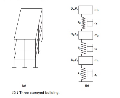
Consider a three storeyed reinforced concrete (RC) building as shown in Fig. 10.1. One can replace the distributed mass or inertia of the system by a finite number of lumped masses or rigid bodies. The masses are assumed to be connected by mass-less elastic damping members. Linear or angular coordinates are used to describe the motion of the lumped masses. Such models are called lumped parameter, lumped mass or discrete mass systems. The minimum number of coordinates necessary to describe the deformed shape of the structure is called the generalized degrees of freedom. Considering the three storeyed RC building as shown in Fig. 10.1a suggests a three degree lumped-mass model as indicated in Fig. 10.1b.
Another popular method of approximating a continuous system as an MDOF system involves replacing the geometry of the system by a large number of elements. By assuming a simple solution within each element, the principle of compatibility and equilibrium are used to find the approximate solution to the original system. This method is the finite element method, which will be discussed later.
Equations of motion of an MDOF system
Consider a three storeyed building modelled as shown in Fig. 10.1b. If one wants to study the dynamic behaviour of a multi-storey frame in the x direction one can consider the generalized coordinates U1, U2, U3 as shown.
Consider the free body diagram of three masses as shown in Fig. 10.2 and applying DŌĆÖAlembertŌĆÖs principle, the equations of motion are written as
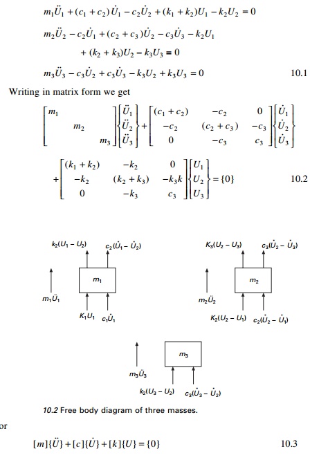
where [m] = mass matrix [c] = damping matrix [k] = stiffness matrix
If the system has n degrees of freedom, the size of [m], [c] and [k] is n ├- n.
ŌĆó Mass matrix: There are two ways of forming the mass matrix of the structure: lumped mass and consistent mass. The mass matrix shown in Eq. 10.2 is a lumped mass matrix. If we consider rotational degrees of freedom, rotary inertia must be considered. The consistent mass matrix is fully populated whereas lumped mass matrix is diagonal.
ŌĆó Stiffness matrix: The stiffness matrix [k] is symmetric. The total stiffness matrix will be formed by assembling all the elements together to form a structure. The stiffness matrix for dynamic analysis is to be calculated by using standard structural application procedures.
ŌĆó Damping matrix: The damping values are to be obtained experimentally. Usually a concrete structure has 5% of critical damping and steel structure and 2% of critical damping. [c] matrix will be reduced to simpler forms to facilitate the analysis.
ŌĆó Load vector: The dynamic loads are assumed to act at nodal points.
Free undamped vibration of an MDOF system
The equation of motion for an undamped system can be written as
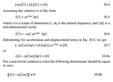
The determinant is known as frequency determinant or characteristic equation. Equation 10.7 can also be written as

Hence for a non-trivial solution to exist the determinant of the following matrix must be equal to zero

Equation 10.8b leads to the nth order nonlinear equation in terms of Žē n2 whereas Eq. 10.10 involves the nth order nonlinear equation in terms of 1/Žē n2 . Equation 10.9 is also written as

where [D] = [k]-1[m] = [a][m] is known as the dynamic matrix. Equation 10.12 is in the form of a typical eigenvalue problem. The vector {Žł} is called an eigenvector and ╬╗ = 1/ Žē n2 is called the eigenvalue.
One of the various ways of obtain the solution is to make the following determinant zero.

The determinant with respect to eigenvalue is plotted in Fig. 10.3.
The solution of the polynomial equation Eq. 10.14 is known as characteristic equation or frequency equation that will yield n values of ╬╗. Once ╬╗ are
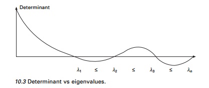
determined {Žł} can be determined. It may be noted that a unique solution for {Žł} does not exist. We obtain only the ratios among {Žł}s.
Orthogonality relationship
For an MDOF system if Žē n( r ) , Žē n( s ) are two natural frequencies, {Žł}(r), {Žł}(s) are the corresponding modal vectors.
For the rth mode Eq. 10.7 can be written as
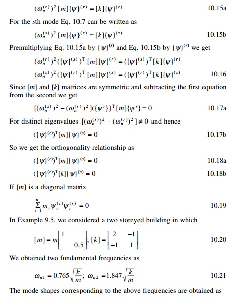
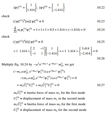
Equation 10.27 can then be interpreted as the work done by inertia forces occurring in the first mode in going through displacements of the second mode are equal to zero. This is known as the orthogonality relationship.
Normalization of modes
It has been seen that the normal modes indicate the ratio between displacements. As such, the different elements may be varied in such a way that a constant ratio is maintained. There are an infinite numbers of such possibilities. Scaling of the normal modes is sometimes done to standardize their elements associated with amplitudes in various degrees of freedom which is known as normalization. For example for the two storey frame discussed

Let us normalize the vector {Žł}(0) by dividing each of the elements by M1 and call it as {Žå}(1) denoted as the normalized eigenvector corresponding to first mode. It is given by
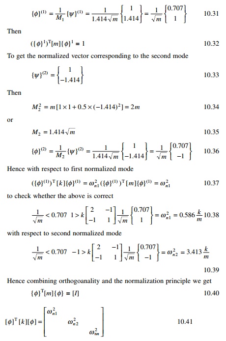
In future chapters we will use a normalized vector {Žå} instead of an eigenvector {Žł}.
Influence coefficient method
The equations of motion of an MDOF system can also be written in terms of influence coefficients which are extensively used in structural engineering. Basically one set of influence coefficients can be associated with each of the matrices involved in the equation of motion. For some problems it is easier to find the flexibility matrix (inverse of stiffness matrix) rather than the stiffness matrix.
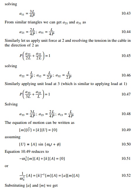
Assume three masses are attached to a string as shown in Fig. 10.4. The tension in the string can be assumed to be equal to P. We can develop dynamic equation of equilibrium as shown below.
First develop the flexibility matrix. The flexibility influence coefficient aij is defined as the deflection at ŌĆśiŌĆÖ due to unit force at ŌĆśjŌĆÖ. Apply unit force at 1, the vertical displacement at 1 is found out by resolving the tension in the direction of 1 as

For a non-trivial solution to exist, the determinant of the above matrix should be equal to zero.
The characteristic equation is
For civil engineering problems all roots are real. If roots are real one can apply CordonŌĆÖs solution to find the roots of a characteristic equation if it is cubic.
1 CordonŌĆÖs solution
Consider the following cubic equation
╬╗3 + b╬╗2 + c╬╗ + d = 0 ,,,, ,,,, 10.67
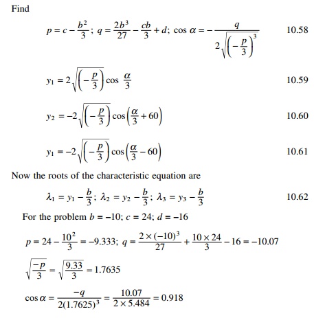
╬▒ = 0.407rad = 23.346┬ o
y1 = 2 ├- 1.7635 cos (0.407/3) = 3.527
Y2 = -2 ├- 1.7635 cos [(0.407 + ŽĆ)/3] = 2
Y2 = 2 ├- 1.7635 cos [(0.407 + ŽĆ)/3] = 1.16
╬╗1 = y1 - b/3 = 3.527 + 3.33 = 6.85
╬╗2 = y2 - b/3 = -1.33 + 3.33 = 2 ╬╗3 = y3 - b/3 = -2.17 + 3.33 = 1.16
Check ╬╗1 + ╬╗2 + ╬╗3 = 10 = 3 + 3 + 4 = trace of the matrix.

We can get the characteristic equation and the solution of the characteristic equation using MATHEMATICA as shown below.
Program 10.2: MATLAB program to find the frequencies and normalized mode shapes
% program to get normalized vectors and eigen values
clc;
close all;
m=[1 0 0;0 1 0;0 0 1];
disp(ŌĆś mass matrixŌĆÖ)
m
%you can give stiffness matrix
% disp(ŌĆś stiffness matrixŌĆÖ)
% k=[2 -1 0;-1 2 -1;0 -1 1];
% k
% a=inv(k);
% or you can given flexibility matrix directly
a=[.75 .5 .25;.5 1 .5;.25 .5 .75]; disp(ŌĆś flexibility matrixŌĆÖ)
a c=a*m;
[ms,ns]=size(m);
%eigen values and eigen vectors [V,D]=eig(c);
for i=1:ms e(i)=1/D(i,i);
end Qh=max(e)+0.001; Ql=0;
for i=1:ms for j=1:ms
if e(j) > Ql & e(j) < Qh kk=j;
Qh=e(j); else
end end Ql=Qh;
Qh=max(e)+0.001;
om1(i)=e(kk);
omega(i)=sqrt(e(kk)); for l=1:ms
p1(l,i)=V(l,kk); end
end
%Normalizing the mode shape L=p1'*m*p1;
%develop modal matrix for i=1:ms
for j=1:ms p(i,j)=p1(i,j)/sqrt(L(j,j));
end end
disp(ŌĆś Natural frequencies in rad/secŌĆÖ) disp(omega)
disp(ŌĆś normalized modal vectorŌĆÖ) disp(p)
pŌĆÖ*m*p
OUTPUT
mass matrix
m =
1 0 0
0 1 0
0 0 1
a =
0.7500 0.5000 0.2500
0.5000 1.0000 0.5000
0.2500 0.5000 0.7500
Natural frequencies in rad/sec
0.7654 1.4142 1.8478
normalized modal vector
0.5000 -0.7071 -0.5000
0.7071 0.0000 0.7071
0.5000 0.7071 -0.5000
ans = proof of normality principle
1.0000 0.0000 0.0000
0.0000 1.0000 0.0000
0.0000 0.0000 1.0000
Example 10.1
Determine the stiffness matrix and write the dynamic equation of equilibrium for the frame shown in Fig. 10.6. Neglect the effect of axial stiffness of the members AB, BC and CD.
Solution
In total there are six degrees of freedom, three at B and three at C. But we neglect axial deformations in all the three members.
Generalized coordinate = total coordinates - constraint equations = 6 - 3 = 3
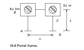
The three generalized coordinates are q1, q2, the rotations at B and C and horizontal sway q3 at C. For every member let us consider the moment stress resultants as shown in Fig. 10.7.
The deformations are denoted by ╬┤. We can establish the compatibility matrix which gives relationship between deformations and generalized coordinates (see Fig. 10.8)
{╬┤} = [╬▓]{q}
The first, second and third columns of [╬▓] matrix are established by applying unit values for the generalized coordinates as
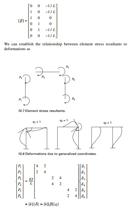
From the principle of virtual work it can be proved that the generalized forces are written in terms of element stress resultants as
{Q} = [╬▓]t{p} = [╬▓]t[k][╬▓] = [K]{q}
so the structural stiffness matrix can be written in terms of element stiffness matrix as

The stiffness matrix could also be obtained straight away by applying the influence coefficient method.
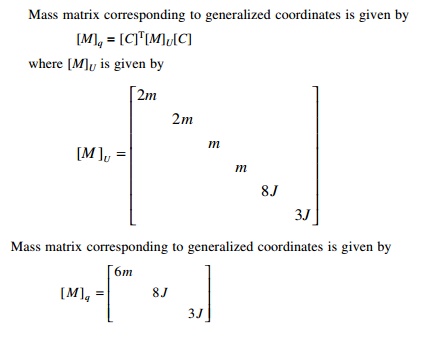
The mass matrix is given by

Hence dynamic equilibrium equations can be written as
[ M ]{q˙˙} + [ K ]{q} = {Q}
Since the structure has three degrees of freedom, CordonŌĆÖs solution can be applied to evaluate the frequencies and mode shapes.
Example 10.2
Determine the stiffness matrix and dynamic equation of equilibrium for the frame shown in Fig. 10.9. Neglect axial deformations.
Solution
Let us consider total six displacements, three at each node B and C as shown in Fig. 10.9d.
Generalized coordinates = total coordinates - constraint equations
= 6 - 3 = 3
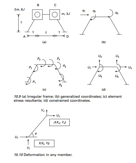
viz. q1, q2, q3.
Consider any member IJ as shown in Fig. 10.10. Axial deformation can be written as
ŌłåIJ = (UJ - UI)C + (VJ - VI)S
Where
We can write the three constraint equations corresponding to axial deformations of the three members as
ŌłåAB = l(U1 + U3) = 0
ŌłåBC = L(U2 - U1) + 0(U4 - U3) = 0; i.e (U2 - U1) = 0
ŌłåCD = l(-U2 + U4) = 0 i.e. (-U2 + U4) = 0
Writing this in matrix form

Selecting constraint coordinate as U1 , the other three displacements can be written as in terms of constrained coordinate as

solving we get U2 = U1; U3 = -U1; U4 = U1.
We can write relation between constrained coordinates and generalized coordinates as
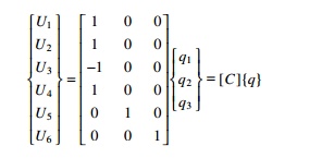
Now we can get the relationship between generalized displacements and deformations (see Fig. 10.11). The relationship between element deformations and generalized displacements is given as (l = 0.707). (Assume lengths of all the members are equal to L = 1).
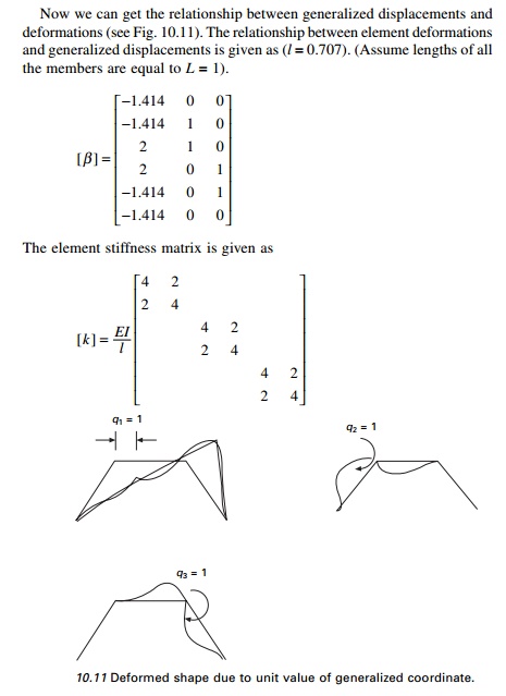
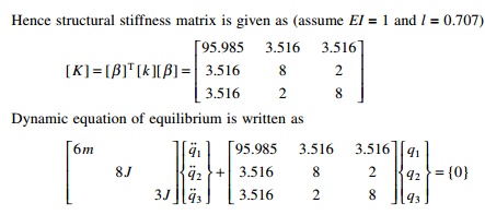
Since there are only three degrees of freedom CordonŌĆÖs solution can be applied to evaluate the frequencies.
10.10 Program 10.3: MATLAB program for solving structural problem by the stiffness method
% Analysis of structures by stiffness method - semi direct approach clc;
clear all; r=input(ŌĆśENTER ├'0├' FOR DATA FROM FILE,├'1├' FOR DATA FROM TERMINAL,├'2├' FOR INTERACTIVEŌĆÖ); ff1=fopen(ŌĆśstout.datŌĆÖ,ŌĆÖwŌĆÖ);
if r<1 ff=fopen(ŌĆśst.datŌĆÖ,ŌĆÖrŌĆÖ); x1=fscanf(ff,ŌĆÖ%sŌĆÖ,1); disp(x1); rb=fscanf(ff,ŌĆÖ%fŌĆÖ,1); cb=fscanf(ff,ŌĆÖ%fŌĆÖ,1); for i=1:rb
for j=1:cb c1=fscanf(ff,ŌĆÖ%fŌĆÖ,1); b(i,j)=c1;
end end disp(b);
x2=fscanf(ff,ŌĆÖ%sŌĆÖ,1); disp(x2); rk=fscanf(ff,ŌĆÖ%fŌĆÖ,1); ck=fscanf(ff,ŌĆÖ%fŌĆÖ,1); for i=1:rk
for j=1:ck c2=fscanf(ff,ŌĆÖ%fŌĆÖ,1); k(i,j)=c2;
end end disp(k);
x3=fscanf(ff,ŌĆÖ%sŌĆÖ,1); disp(x3); rdo=fscanf(ff,ŌĆÖ%fŌĆÖ,1); cdo=fscanf(ff,ŌĆÖ%fŌĆÖ,1); for i=1:rdo
for j=1:cdo c3=fscanf(ff,ŌĆÖ%fŌĆÖ,1); do(i,j)=c3;
end end
disp(do); x4=fscanf(ff,ŌĆÖ%sŌĆÖ,1); disp(x4); rfo=fscanf(ff,ŌĆÖ%fŌĆÖ,1); cfo=fscanf(ff,ŌĆÖ%fŌĆÖ,1);
for i=1:rfo for j=1:cfo
c4=fscanf(ff,ŌĆÖ%fŌĆÖ,1); fo(i,j)=c4;
end end
disp(fo); x5=fscanf(ff,ŌĆÖ%sŌĆÖ,1); disp(x5); rpo=fscanf(ff,ŌĆÖ%fŌĆÖ,1); cpo=fscanf(ff,ŌĆÖ%fŌĆÖ,1); for i=1:rpo
for j=1:cpo c5=fscanf(ff,ŌĆÖ%fŌĆÖ,1); po(i,j)=c5;
end end
disp(po); x6=fscanf(ff,ŌĆÖ%sŌĆÖ,1); disp(x6); rsk=fscanf(ff,ŌĆÖ%fŌĆÖ,1); csk=fscanf(ff,ŌĆÖ%fŌĆÖ,1); for i=1:rsk
for j=1:csk
c5=fscanf(ff,ŌĆÖ%fŌĆÖ,1); ks(i,j)=c5;
end end
disp(ks); else
if r<2
%INPUT FOR BETA MATRIX
b=[-1.414 0 0;-1.414 1 0;2 1 0;2 0 1;-1.414 0 1;-1.414 0 0]; %disp(b);
%INPUT FOR ELEMENT STIFFNESS MATRIX k
k=[4 2 0 0 0 0; 2 4 0 0 0 0;0 0 4 2 0 0;0 0 2 4 0 0;0 0 0 0 4 2;0 0 0 0 2 4]; disp(k);
%INPUT FOR INITIAL STRAIN DO do=[0;0;0;0;0;0];
disp(do);
%INPUT FOR APPLIED FORCE fo=[0;0;0];
disp(fo);
%INPUT FOR INITIAL STRESS pO po=[0;0;0;0;0;0];
disp(po);
%input spring stiffness ks=[0,0,0;0,0,0;0,0,0]; disp(ks);
else
rb=input(ŌĆśNUMBER OF ROWS IN B MATRIXŌĆÖ); cb=input(ŌĆśNUMBER OF COLUMNS IN B MATRIXŌĆÖ); for i = 1:rb
for j = 1:cb
bm = input(ŌĆś ŌĆś); b(i,j)=bm;
end end disp(b);
rk=input(ŌĆśNUMBER OF ROWS IN ELEMENT STIFFNESS MATRIXŌĆÖ); ck=input(ŌĆśNUMBER OF COLUMNS IN ELEMENT STIFFNESS MATRIXŌĆÖ); for i=1:rk
for j=1:ck c2=input(ŌĆśŌĆÖ); k(i,j)=c2; end
end
disp(k);
rdo=input(ŌĆśNUMBER OF ROWS IN INITIAL STRAIN MATRIXŌĆÖ); cdo=input(ŌĆśNUMBER OF COLUMNS IN INITIAL STRAIN MATRIXŌĆÖ); for i=1:rdo
for j=1:cdo c3=input(ŌĆśŌĆÖ); do(i,j)=c3; end
end disp(do);
rfo=input(ŌĆśNUMBER OF ROWS IN APPLIED FORCESŌĆÖ); cfo=input(ŌĆśNUMBER OF COLUMNS IN APPLIED FORCESŌĆÖ); for i=1:rfo
for j=1:cfo c4=input(ŌĆśŌĆÖ); fo(i,j)=c4; end
end disp(fo);
rpo=input(ŌĆśNUMBER OF ROWS IN INITIAL STRESS MATRIXŌĆÖ); cpo=input(ŌĆśNUMBER OF COLUMNS IN INITIAL STRESS MATRIXŌĆÖ); for i=1:rpo
for j=1:cpo c5=input(ŌĆśŌĆÖ); po(i,j)=c5; end
end disp(po); end
end K1=(bŌĆÖ*k*b); K=K1+ks;
ffi=fo-(bŌĆÖ*po)+(bŌĆÖ*k*do); u=inv(K)*ffi;
p=(k*b*u); pf=po+p-(k*do);
q=input(ŌĆśENTER ├'0├' FOR O/P IN FILE,├'1" for O/P IN TERMINALŌĆÖ) ; if q>0
ŌĆśDISPLACEMENTS AT GENERALIZED COORDINATESŌĆÖ disp(u);
ŌĆśELEMENT FORCES DUE TO APPLIED FORCESŌĆÖ disp(p);
ŌĆśFINAL ELEMENT FORCESŌĆÖ
disp(pf); else
fprintf(ff1,ŌĆÖ\r\nDISPLACEMENTS AT GENERALIZED COORDINATESŌĆÖ); fprintf(ff1,ŌĆÖ\r\n%10.4f ŌĆś, u);
fprintf(ff1,ŌĆÖ\r\nELEMENT FORCES DUE TO APPLIED FORCESŌĆÖ); fprintf(ff1,ŌĆÖ\r\n%10.4fŌĆÖ, p);
fprintf(ff1,ŌĆÖ\r\nFINAL ELEMENT FORCESŌĆÖ); fprintf(ff1,ŌĆÖ\r\n%10.4fŌĆÖ,pf);
end
Output
>> K
K =
95.9855 3.5160 3.5160
3.5160 8.0000 2.0000
3.5160 2.0000 8.0000
Static condensation of stiffness matrix
In most of the structural dynamics problems, mass moment of inertia is only included corresponding to translational degrees of freedom. However, a more generalized formulation of stiffness matrix includes terms corresponding to rotational degrees of freedom. It is necessary to eliminate the extraneous degree of freedom associated with rotation from the stiffness matrix. This method is called static condensation. This enables the number of degrees of freedom to be reduced to a desired level.
To establish the equations used in static condensation, assume that [K] and the corresponding force vector are partitioned as
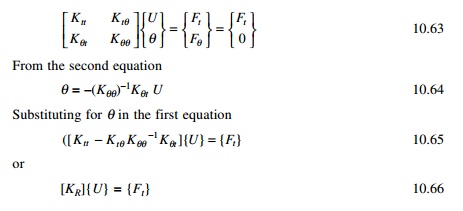
The stiffness is now suitable for use with the lumped mass matrix to write equations of motion for translational vibration. Once translational degrees of freedom are obtained, rotational degrees of freedom can be obtained from Eq. 10.64.
General viscous damping
The differential equation governing the free vibration of an MDOF system with general viscous damping is given by

If the damping matrix is arbitrary, it is somewhat complex to solve the equations. The above equation is reformulated as 2n first order differential equations by writing
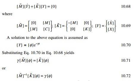
The values of ╬│ occur in complex conjugate pairs. The system is stable only if all eigenvalues have non-negative real parts. Eigenvectors correspond to complex conjugates of one another. Eigenvectors correspond to eigenvalues which are not complex conjugates satisfy the orthogonality relationship

Example 10.3
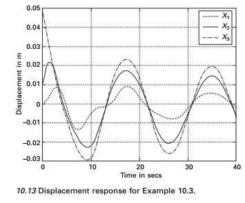
Plot the free vibration response of the shear frame shown in Fig. 10.12 under initial conditions.
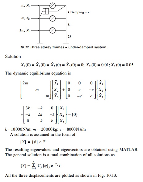
All the three displacements are plotted as shown in Fig. 10.13.
Program 10.4: MATLAB program for free vibration of MDOF with general damping
% FREE VIBRATION OF GENERAL DAMPED THREE DEGREE OF FREEDOM SYSTEM
clc; clear all; digits(5)
% mass matrix disp(ŌĆś mass matrixŌĆÖ)
m=[40000 0 0;0 20000 0;0 0 20000]; m
[ms,ns]=size(m); %damping matrix disp(ŌĆś damping matrixŌĆÖ)
c=[0 0 0;0 -8000 8000;0 -8000 8000]; c
%stiffness matrix disp(ŌĆś stiffness matrixŌĆÖ)
k=[30000 -10000 0;-10000 20000 -10000;0 -10000 10000]; k
z=zeros(ms); MT=[z m;m c]; KT=[-m z;z k]; Z=inv(MT)*(KT); [V,D]=eig(Z); disp(ŌĆś eigenvaluesŌĆÖ) for i=1:2*ms
DS(i)=D(i,i); end
DS
disp(ŌĆś eigenvectorsŌĆÖ) V
disp(ŌĆś initial conditionsŌĆÖ) x0=[0;0;0;0;0.01;0.05];
disp(ŌĆś constants of integrationŌĆÖ) S=inv(V)*x0 tk=linspace(0,40,2001);
%Evaluation of time dependent response %recall that x1=y4; and x2=y5; x3=y6 for k=1:2001
t=tk(k);
for i=ms+1:2*ms x(k,i-ms)=0; for j=1:2*ms
x(k,i-ms)=x(k,i-ms)+(real(S(j))*real(V(i,j))-...
imag(S(j))*imag(V(i,j)))*cos(imag(D(j,j))*t); x(k,i-ms)=x(k,i-ms)+(imag(S(j))*real(V(i,j))-...
real(S(j))*imag(V(i,j)))*sin(imag(V(j,j))*t); x(k,i-ms)=x(k,i-ms)*exp(-real(D(j,j))*t);
end end
end figure(1)
plot(tk,x(:,1),ŌĆÖk├'ŌĆÖ,tk,x(:,2),ŌĆÖkŌĆÖ,tk,x(:,3),ŌĆÖk-.ŌĆÖ) xlabel(ŌĆś t(sec)ŌĆÖ)
ylabel(ŌĆś displacement in mŌĆÖ) gtext(ŌĆś├'├'├'├' x1ŌĆÖ) gtext(ŌĆś______ x2ŌĆÖ) gtext(ŌĆś-.-.-.-.-.x3ŌĆÖ)
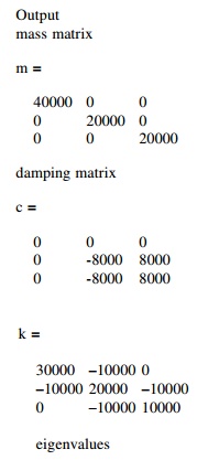
Output mass matrix
ans =
-0.0882 - 1.2170i -0.0882 + 1.2170i 0.0367 - 0.8097i 0.0367 + 0.8097i 0.0516 - 0.3537i 0.0516 + 0.3537i
eigenvectors
V =
0.2012 - 0.0597i 0.2012 + 0.0597i -0.0206 - 0.4559i -0.0206 + 0.4559i -0.0156 - 0.0762i -0.0156 + 0.0762i
-0.6333 -0.6333 0.1004 - 0.1794i 0.1004 + 0.1794i -0.0280 - 0.1935i - 0.0280 + 0.1935i
0.0741 - 0.3841i 0.0741 + 0.3841i 0.3371 + 0.1799i 0.3371 - 0.1799i - 0.0379 - 0.2600i -0.0379 + 0.2600i
0.0608 + 0.1609i 0.0608 - 0.1609i 0.5630 0.5630 0.2172 - 0.0124i 0.2172 + 0.0124i
-0.0375 - 0.5177i -0.0375 + 0.5177i 0.2155 + 0.1337i 0.2155 - 0.1337i 0.5470 + 0.0005i 0.5470 - 0.0005i
0.3184 + 0.0378i 0.3184 - 0.0378i -0.2405 + 0.4054i -0.2405 - 0.4054i 0.7349 0.7349
initial conditions x0 =
0
0
0
0
0.0100
0.0500
constants of integration
S =
0.0049 - 0.0109i
0.0049 + 0.0109i -0.0135 - 0.0058i -0.0135 + 0.0058i 0.0237 + 0.0317i 0.0237 - 0.0317i
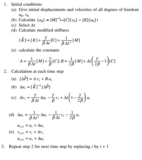
NewmarkŌĆÖs numerical integration
In 1959, N M Newmark developed a family of time stepping methods. The method discussed for the SDOF system in Chapter 7 may be extended to the MDOF system.
Algorithm
ŌĆó Average acceleration method ╬│ = 1/2; ╬▓ = 1/4
Linear acceleration method ╬│ = 1/2; ╬▓ = 1/6
3. Repeat step 2 for next time step by replacing i by i + 1
Program 10.5: MATLAB program for NewmarkŌĆÖs method of MDOF with generalized damping
%free vibration of mdof system damped using newmarkŌĆÖs method
%mass matrix
clc; close all;
m=[40000 0 0;0 20000 0;0 0 20000]; disp(ŌĆś mass matrixŌĆÖ)
m
%damping matrix
c=[0 0 0;0 8000 -8000;0 -8000 8000]; disp(ŌĆś damping matrixŌĆÖ)
c
%stiffness matrix
k=[30000 -10000 0;-10000 20000 -10000;0 -10000 10000]; k
%specify integration parameters for linear acceleration method
%beta=1/6;
%gamma=0.5;
%specify integration parameters for constant acceleration method beta=1/4;
gamma=0.5;
%specify increment in time dt=0.002;
%calculate the following constants b1=1/(beta*dt^2);
%b2=1/(beta*dt);
%b3=beta-0.5;
b4=gamma*dt*b1;
%b5=1+gamma*dt*b2;
%b6=dt*(1+gamma*b3-gamma); kt=k+b1*m+b4*c; ad=(1/(beta*dt))*m+(gamma/beta)*c;
bd=(1/(2*beta))*m+dt*(gamma/(2.0*beta)-1)*c; %specify initial displacements
u0=[0 0.01 0.05]ŌĆÖ; v0=[0 0 0]ŌĆÖ;
a0=inv(m)*(-c*v0-k*u0); t(1)=0;
for i=1:3 u(i,1)=u0(i); v(i,1)=v0(i); a(i,1)=a0(i); end
for i=2:20000 t(i)=(i-1)*dt; for j=1:3
uu(j)=u(j,i-1); vv(j)=v(j,i-1);
aa(j)=a(j,i-1); end
fba=(ad*vvŌĆÖ+bd*aaŌĆÖ); kti=inv(kt); up=kti*fba;
vp=(gamma/(beta*dt))*up-(gamma/beta)*vvŌĆÖ+(1-gamma/(2.0*beta))*aaŌĆÖ; ap=b1*up-(1/(beta*dt))*vvŌĆÖ-(1/(2.0*beta))*aaŌĆÖ;
for j=1:3 u(j,i)=u(j,i-1)+up(j); v(j,i)=v(j,i-1)+vp(j); a(j,i)=a(j,i-1)+ap(j);
end end figure(1)
plot(tŌĆÖ,u(1,:)ŌĆÖ,ŌĆÖ-ŌĆÖ,tŌĆÖ,u(2,:)ŌĆÖ,ŌĆÖkŌĆÖ,tŌĆÖ,u(3,:)ŌĆÖ,ŌĆÖ-.ŌĆÖ) gtext(ŌĆś- - x1ŌĆÖ)
gtext(ŌĆś___x2ŌĆÖ) gtext(ŌĆś-.-. x3ŌĆÖ)
When Example 10.3 is solved by NewmarkŌĆÖs method we get the response as shown in Fig. 10.14.
Forced response of a three-degrees-of-freedom under-damped system
Consider forced vibration of a three-degrees-of-freedom under-damped system as shown in Fig. 10.1b. The equation of motion is written in matrix form as
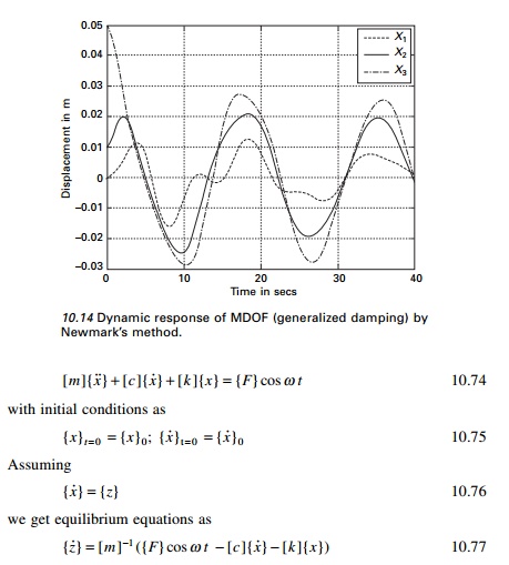
Combining Eq. 10.76 and 10.77 we get six first order linear differential
equations and they are solved using the Runge-Kutta method as explained in Previous Pages.
As an example consider
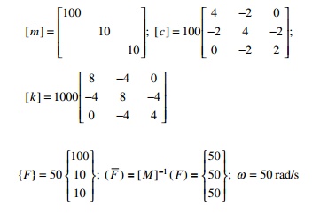
A MATLAB listing of the program is given below and the displacement response is shown in Fig. 10.15.
Program 10.6 MATLAB program for forced vibration of three degrees of freedom by RungeŌĆ'Kutta method
% three degrees of freedom forced vibration by rk method clc;
tspan=[0:.01:10];
y0=[0;0;0;0;0;0]; [t,y]=ode45(ŌĆśdfunc3fŌĆÖ,tspan,y0); subplot(311)
plot(t,y(:,1)); xlabel(ŌĆśtŌĆÖ); ylabel(ŌĆśx1(t)ŌĆÖ); title(ŌĆś x1(t) vs tŌĆÖ);
subplot(312)
plot(t,y(:,3)); xlabel(ŌĆśtŌĆÖ); ylabel(ŌĆśx2(t)ŌĆÖ); title(ŌĆśx2(t) vs tŌĆÖ); subplot(313) plot(t,y(:,5)); xlabel(ŌĆśtŌĆÖ); ylabel(ŌĆśx3(t)ŌĆÖ); title(ŌĆśx3(t) vs tŌĆÖ)
function f=dfunc3f(t,y)
% four first order equations are given by f f=zeros(6,1);
%mass matrix m=[100,0,0;0,10,0;0,0,10]; %damping matrix
c=[400,-200,0;-200,400,-200;0,-200,200]; %stiffness matrix k=1000*[8,-4,0;-4,8,-4;0,-4,4];
%give forces force=50*[1;1;1]; om=5.0;
%four first order equations f(1)=y(2);
f(2)=force(1)*cos(om*t)-c(1,1)*y(2)/m(1,1)-c(1,2)*y(4)/m(1,1)...
-c(1,3)*y(6)/m(1,1)-k(1,1)*y(1)/m(1,1)-k(1,2)*y(3)/m(1,1)-k(1,3)*y(5)/ m(1,1);
f(3)=y(4); f(4)=force(2)*cos(om*t)-c(2,1)*y(2)/m(2,2)-c(2,2)*y(4)/m(2,2)...
-c(2,3)*y(6)/m(2,2)-k(2,1)*y(1)/m(2,2)-k(2,2)*y(3)/m(2,2)-k(2,3)*y(5)/m(2,2); f(5)=y(6); f(6)=force(3)*cos(om*t)-c(3,1)*y(2)/m(3,3)-c(3,2)*y(4)/m(3,3)...
-c(3,3)*y(6)/m(3,3)-k(3,1)*y(1)/m(3,3)-k(3,2)*y(3)/m(3,3)-k(3,3)*y(5)/m(3,3)
Summary
The vibration of an n-degree-of-freedom system is governed by a system of n differential equations. The general solution of these differential equations is the sum of a homogeneous solution and a particular solution. The homogeneous solution is the free vibration response, and its determination is often necessary before the forced response can be determined. The free vibration analysis of an MDOF system is significantly more complicated than the free vibration analysis of a one or two-degrees-of-freedom system.
Related Topics