Chapter: Civil : Structural dynamics of earthquake engineering
Forced vibration (harmonic force) of single-degree-of-freedom systems
Forced
vibration (harmonic force) of single-degree-of-freedom systems in relation to
structural dynamics during earthquakes
Abstract: In this
chapter, forced vibration of single-degree-of-freedom (SDOF) systems
(both undamped and under-damped) due to harmonic force is considered. Governing
equations are derived and the displacement response is determined using
WilsonŌĆÖs recurrence formula. Vibration excitation due to imbalance in rotating
machines is discussed. Equations for transmissibility are derived for force and
displacement isolation. The underlying principle of vibration-measuring
instruments is illustrated.
Key words: resonance, transient, steady
state, magnification factor, beating, transmissibility, seismometer,
accelerometer.
Forced vibration without
damping
In many important vibration
problems encountered in engineering work, the exciting force is applied
periodically during the motion. These are called forced vibrations. The
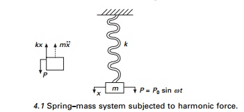
most common periodic force is a harmonic force of time such as
P = P0 sin
Žēt ŌĆ”ŌĆ”ŌĆ”ŌĆ” 4.1
where P0 is a constant, Žē is the forcing frequency and t
is the time. The motion is analysed using Fig. 4.1.

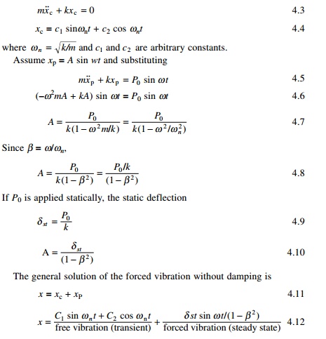
The general solution of Eq. 4.2 (non-homogeneous second order
differential equation) consists of two parts x = xc + xp
where xc = complementary solution,
and xp = particular solution. The
complementary solution is obtained by setting right hand side as zero.
The first two terms of free
vibration are dependent only on properties m and k of the system
and also on initial conditions. This is called transient vibration because,
in a real system, it is damped out by friction.
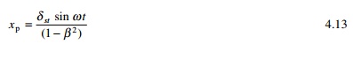
The third term represents forced
vibration and depends on the amplitude of applied force and forcing frequency Žē (or ╬▓ = Žē/Žēn). This
is called steady state vibration since it is the motion of the
system after a transient vibration is dissipated.
Resonance:
Steady
state vibration
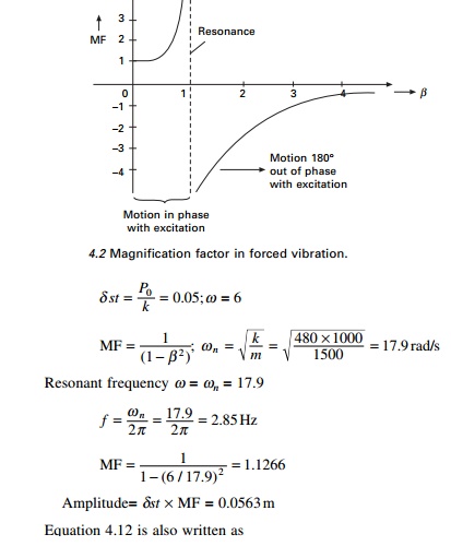
The amplitude is ╬┤st/(1 ŌĆ' ╬▓ 2) and it becomes
infinite when ╬▓ = 1.
This condition is called resonance.
Of course the amplitude does not become infinity in practice
because of damping or physical constraints but the condition is a dangerous
one, causing fractures. We define magnification factor as
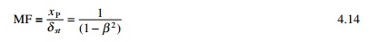
and it is plotted as shown in
Fig. 4.2. Several items are of particular interest in this diagram.
Example 4.1
A 1500 kg truck cab is assumed to
be supported by four springs each with stiffness 120 kN/m. Determine the
resonant frequency of the cab in unit of Hz and the amplitude of vibration if
the displacement input of each accelerator is d = 0.05 sin 6t.
Solution
We know that
mx╦Ö╦Ö + kx = P0 sin Žē t
m = 1500
kg; k = 4 ├- 120 ├- 1000 = 480 ├- 1000
P0 = k╬┤ = 480 ├- 1000 ├- 0.05 = 24
000 N
Substituting in the above equation,
1500 ╦Ö╦Öx + 480 ├- 1000 x = P0
sin 6t
Equation 4.12 is also written as
x = X sin (Žēnt + Žå) + ╬┤st sin (Žēt)/(1ŌĆ' ╬▓2) ŌĆ”ŌĆ”ŌĆ”
ŌĆ”. 4.15
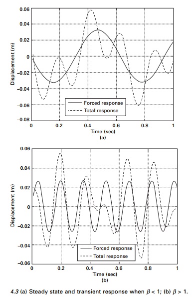
Three distinct types of motion
are possible depending on whether the value of frequency ratio ╬▓ is less than, equal to or
greater than 1.
If ╬▓ <1 then Žē < Žēn
indicating that the natural frequency response (transient) is greater than
forced response (steady state). The resulting motion is represented in Fig.
4.3a. The free vibration portion of the motion completes several cycles in the
time required for one cycle of the forced response. The total motion (depicted
by dotted line) exhibits a sinusoidal variation about a lower frequency base
curve (represented by the solid line in Fig. 4.3a. In this case the forced
response is greater than the equivalent static deflection ╬┤st.
When the frequency ratio ╬▓ > 1 then Žēn < Žē and the total motion is
characterized as the forced response oscillating about the free vibration
portion of the response as indicated in Fig. 4.3b. Also if ╬▓ > 2 , the amplitude of the
forced response will be less than the equivalent static deflection ╬┤st.
![]()
Example 4.2
The undamped springŌĆ'mass system
has a mass of 4.5 kg and a spring stiffness of 3500 N/m. It is excited by a
harmonic force having an amplitude F0 =100 N and an
excitation frequency of Žē =10
rad/s. The initial conditions are x(0) = 0.015 m and v(0) = 0.15
m/s. Determine (a) the frequency ratio (b) the amplitude of the forced
response (c) the displacement of the mass at time t = 2 s. and (d) the velocity
of mass at time t = 4 s. Draw the forced response and total
response curves. If the excitation frequency is 40 r/s determine how the forced
response and total response curves change.
Solution
The natural frequency of the system is calculated as
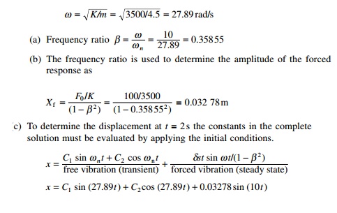
Using the
initial conditions x(0) = 0.015 m and v(0) = 0.15 m/s we get
C 2 = 0.015;
C1 = 0.004 20
Substituting these values in displacement equation and t
= 2 s, we get x (t = 2) = 0.037 79m and v(t = 2) =
0.2270 m/s. The harmonic response of an undamped single-degree-of-freedom
(SDOF) system to harmonic excitation for this problem is shown in Fig. 4.3a.
When the excitation frequency is 40 rad/s then ╬▓ = 1.434; the harmonic response
is shown in Fig. 4.3b.
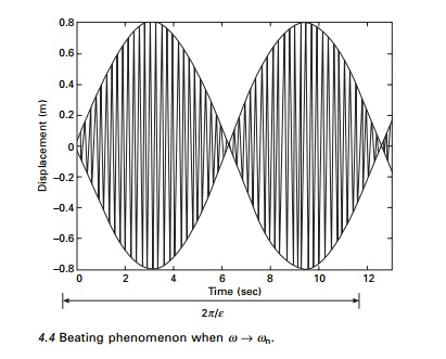
Beating phenomenon
Two very important phenomena occur when the frequency of the
forcing function Žē
approaches natural circular frequency of the system Žēn or when ╬▓ Ōå'
1. First consider Žē and Žēn are
nearly the same or Žēn is
slightly greater than Žē.
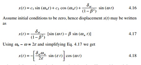
Žē is much
larger than ╬Ą in the
term sin (╬Ąt) and
oscillates with much larger period than cos (Žēt) does. The resulting motion,
illustrated in Fig. 4.4, is a rapid oscillation with slowly varying amplitude
and referred to as beat. Sometimes the two sinusoids add to each other,
and at other times they cancel each other out, resulting in a beating
phenomenon.
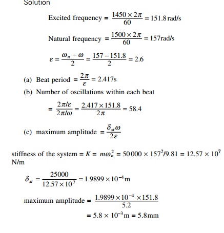
Example 4.3
An undamped system is harmonically forced resulting in a
beating condition. The natural and excited frequencies are 1500 cycles/min and
1450 cycles/ min respectively. Determine (a) beat period (b) number of
oscillations in each beat and (c) the maximum amplitude of oscillation if W
= 50 kN and the amplitude of steady state force is 25 kN.
Resonance
When the excited frequency is exactly equal to the natural
circular frequency we get a condition known as resonance. At this point ╬▓ = 1 and the amplitude of
vibration increases without bound. For this the solution given in Eq. 4.16 is
no longer valid. The particular solution for the equation Eq. 4.5 now is
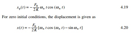
The first term is predominant and
the amplitude varies linearly with respect to time as shown in Fig. 4.5.
Example 4.4
An SDOF system has a total weight
of 5 kN and a spring stiffness of 360kN/ m. The system is excited at resonance
by a harmonic force of 3 kN. Determine the displacement amplitude of the forced
response after (a) 1.25 cycles and
(b) 10.25 cycles.
Solution
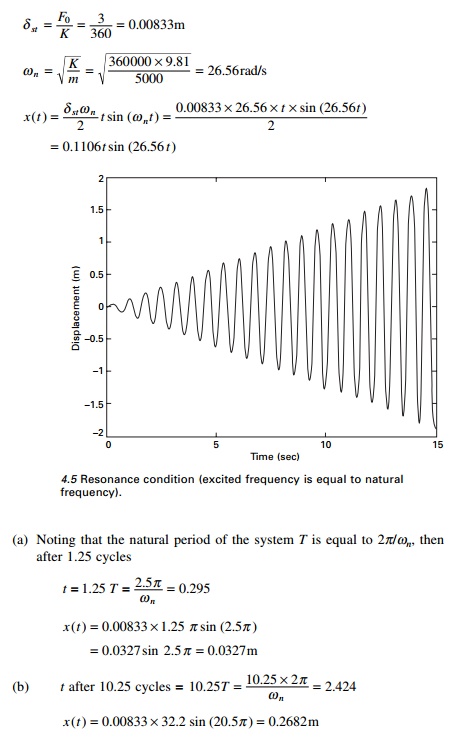
Equation 4.19 indicates that for a system operating at
resonance, the amplitude of the forced response increases linearly with time by
ŽĆ╬┤st per
cycle as indicated in Fig. 4.5. Theoretically, the amplitude will eventually
approach infinity. In reality, however, the system will break down once the
amplitude becomes intolerably large for the structure. Fortunately, since the
steady state amplitude varies directly with time, the system would have to
operate at resonance for an extended period before the amplitude becomes
destructively large. Therefore, it is acceptable for a system or a machine in
route to its operating frequency to quickly pass through the resonance
amplitude.
Forced vibration with
damping
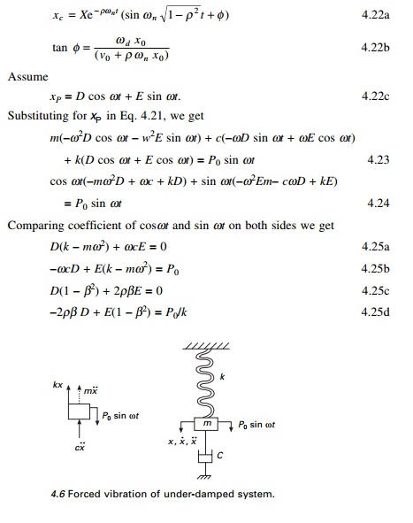
Consider a forced vibration of the under-damped system shown
in Fig. 4.6. The dynamic equilibrium equation is written as,
Equation 4.21 is a second order non-homogeneous equation and
it has both a complementary solution xc and a particular
solution xP . xc is same as that for free
vibration of an under-damped system.
and the plot of MF is shown in Fig. 4.7.
The dramatic increase in MF near
the natural frequency Žēn is
called resonance and Žē is called the resonance
frequency. The following items are of interest in the diagram.
┬Ģ Static
loading: Žē = 0;╬┤/P0 /k = 1. It is independent of damping.
ŌĆó Resonance: Žē = Žēn the
amplitude is magnified substantially when the coefficient of viscous
damping Žü is low.
ŌĆó High-frequency
excitation: Žē >>
Žēn; ╬┤/╬┤st 0 the
mass is essentially stationary because of its inertia of any damping of
motion.
ŌĆó Large
coefficient of viscous damping: The amplitude of the vibration
is reduced at all values of (Žē/Žēn) as the
coefficient of viscous damping Žü is increased in a particular system.
Recurrence formula of Wilson
The recurrence formula is derived in a similar way to that of
free vibration of an under-damped system. The displacement is given in terms of
Eq. 4.30. The displacement x is written as
(where the functions C and S are defined in
Chapter 3) and co = cos (Žēt); si = sin (Žēt) where Žē is the excited frequency.
Differentiating with respect to time t we get velocity expression as

The constants D and E are given in Eq. 4.25e and
f respectively.
For the initial conditions of displacement and velocity the
displacement at any time is given as
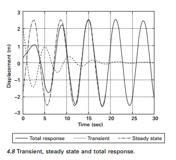
Apart from the last two terms other terms belong to transient
part and the last two terms to steady state. Figure 4.8 shows the transient,
steady state and total response for forced vibration of under-damped SDOF
system.
Program 4.2: MATLAB
program for finding response due to harmonic force
clc close all
%****************************************************
%give mass of the system m=6;
%give stiffness of the system
k=8;
wn=sqrt(k/m);
%give damping coefficient c1=2;
%give initial conditions -
displacement and velocity u(1)=.25;
udot(1)=.5;
%give
magnitude of harmonic force
f=4;
%give excited frequency of the
force w=1;
%****************************************************
beta=w/wn;
cc=2*sqrt(k*m);
rho=c1/cc; wd=wn*sqrt(1-rho^2);
wba=rho*wn; rhoba=rho/sqrt(1-rho^2); b0=2.0*rho*wn; b1=wd^2-wn^2;
b2=2.0*wba*wd; dt=0.02;
t(1)=0;
for i=2:1500 t(i)=(i-1)*dt;
s=exp(-rho*wn*t(i))*sin(wd*t(i));
c=exp(-rho*wn*t(i))*cos(wd*t(i)); sdot=-wba*s+wd*c; cdot=-wba*c-wd*s;
sddot=-b1*s-b2*c; cddot=-b1*c+b2*s; a1=c+rhoba*s;
a2=s/wd; d=-2.0*f*(rho*beta)/(k*(1-beta^2)^2+(2*rho*beta)^2);
e=f*(1-beta^2)/(k*(1-beta^2)^2+(2*rho*beta)^2);
u(i)=a1*u(1)+a2*udot(1)-d*(c+wba*s/wd)-e*w*s/wd;
v(i)=d*(cos(w*t(i)))+e*sin(w*t(i));
x(i)=u(i)+v(i); end
figure(1);
plot(t,x,ŌĆśkŌĆÖ); xlabel(ŌĆś timeŌĆÖ);
ylabel(ŌĆś displacement ŌĆÖ); title(ŌĆś
displacement - timeŌĆÖ);
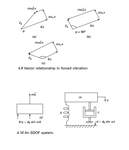
Vector relationship
in forced vibration
For small values of Žē/Žēn <<
1, both inertia and damping forces are small, which results in a small phase
angle Žł. The
magnitude of the impressed force is then nearly equal to the spring force as
shown in Fig. 4.9a. For Žē/Žēn = 1, the
phase angle is 90┬ o and the force diagram
appears as in Fig. 4.9b. The inertia force, which is now larger, is balanced by
the spring force; whereas the impressed force overcomes the damping force. The
amplitude at resonance can be found from Eq. 4.29a. At large values of Žē/Žēn > 1
the phase angle approaches 180┬ o and the
impressed force is expended almost entirely in overcoming the large inertia
force as shown in Fig. 4.9c
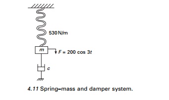
Example 4.5
An SDOF system shown in Fig. 4.10 is modelled as 3000kg mass
on a spring stiffness k = 400 kN/m. The system has a damping factor of c/cc=
0.4. Assume that the spring is attached to the base whose vertical displacement
are defined by d = 0.04 sin 6t. Write the equation of motion of m
for steady
vibration. Determine the magnification factor of the amplitude
of vibration, the amplitude A and phase angleŽł.

Example 4.6
A weight attached to a spring of stiffness 530 N/m and
undergoes viscous damping and the weight was displaced and released as shown in
Fig. 4.11.
The period of vibration was found
to be 1.8 seconds. The ratio of consecutive amplitudes was found to be 4.2/1.
Determine the amplitude and phase angle when a force of 200 cos 3t acts
on the system.
Solution
Given k = 530 N/m; t = 1.8 seconds; (xn+1/xn)
= 4.2
Logarithmic decrement = loge 4.2 = 1.435
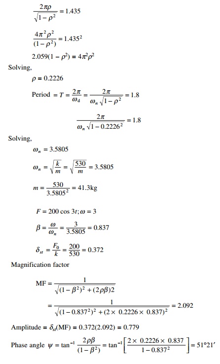
Hence XP = 0.779 sin (3t ŌĆ' Žł) is a steady state.
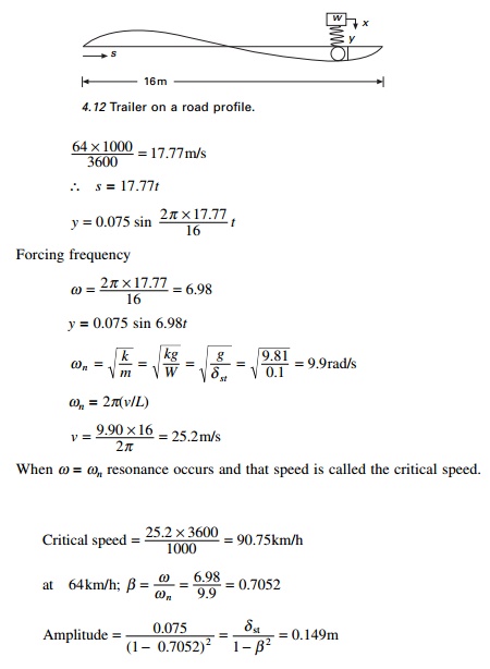
Example 4.7
The spring of an automobile
trailer shown in Fig. 4.12 is compressed under its weight by 100mm. Find the
critical speed when the tractor is travelling over a road with a profile
approximated by a sine wave of amplitude 75mm and a wavelength of 16m. What
will be the amplitude of vibration at 64 km/h? Neglect damping.
Solution
Profile of the road = y = 0.075 sin (2ŽĆs/16)
The equation of motion mx╦Ö╦Ö + k ( x Ōł'
y) = 0 or mx˙˙ + kx = ky
╦Ö╦Öx + Žē n2 ╬┤x = Žē n2 y
s = distance covered = vt
Rotating imbalance
Imbalance in rotating machines is
a common source of vibration excitation. Let us consider a springŌĆ'mass system
constrained to move in the vertical direction and excited by a rotating machine
that is unbalanced as shown in Fig. 4.13. The imbalance is represented by an
eccentric mass m with eccentricity e rotating with angular
velocityŽē.
Let x be the displacement of the non-rotating mass (MŌĆ'm)
from the static equilibrium position, and the displacement of m is
x + e sin Žēt
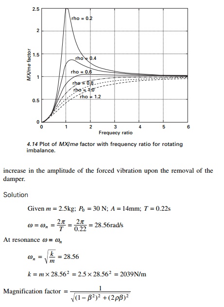
The equation of motion is
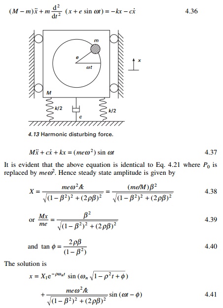
MX/me versus
frequency is plotted in Fig. 4.14 for various damping ratios. The phase
angle with respect to frequency ratio for various damping values is the same as
in Fig. 4.7.
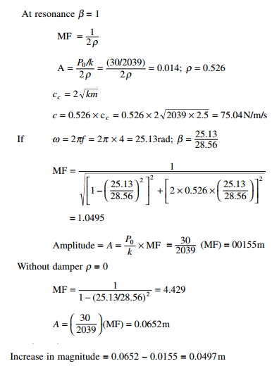
Example 4.8
A machine part having a mass of
2.5kg vibrates in a viscous medium. A harmonic exciting force of 30N acts on
the part and causes resonant amplitude of 14 mm with a period of 0.22s. Find
the damping coefficient. If the frequency of the exciting force is changed to 4
Hz, also determine the increase in the amplitude of the forced vibration upon
the removal of the damper.
Solution
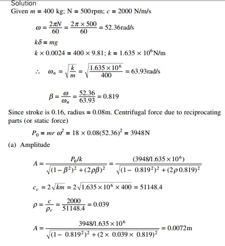
Example 4.9
A single cylinder vertical diesel
engine has a mass of 400kg and is mounted on a steel chassis frame. The static
deflection owing to the weight of the chassis is 2.4mm. The reciprocating mass
of the engine is 18kg and the stroke of the engine is 160 mm. A dashpot with a
damping coefficient of 2N/mm/s is also used to dampen the vibration. In the
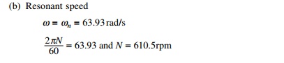
steady state of vibration, determine (a) the amplitude of the vibration if the
driving shaft rotates at 500 rpm and (b) the speed of the driving shaft when
the resonance occurs.
Solution
Given m = 400 kg; N = 500rpm; c = 2000 N/m/s
Example 4.10
A body having a mass of 15kg is
suspended from a spring which deflects 12mm under the weight of the mass.
Determine the frequency of free vibration and also the viscous damping force
needed to make the motion periodic or a speed of 1mm/s.
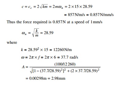
When dampened to this extent, a
disturbing force having a maximum value of 100N and vibrating at 6Hz is made to
act on the body. Determine the amplitude of ultimate motion.
Solution
Given 15kg; ╬┤st = 12mm; P0 =
100N; f = 6Hz
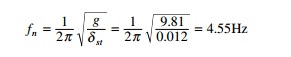
The motion becomes a periodic when the damped frequency is
zero or when it is critically damped, i.e. Žü = 1 and Žē = Žēn = 2ŽĆf = 2ŽĆ ├- 4.55 =
28.59 rad/s
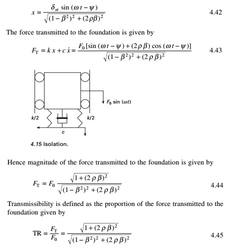
Transmissibility
(force isolation)
Consider the springŌĆ'massŌĆ'damper
system subjected to harmonic force shown in Fig. 4.15 which is generated by
machines and engines. These vibrations are often unavoidable; however, their
effect on a dynamical system can be reduced significantly by properly designed
springs and damper system known as isolators.
We know that the displacement response is given by
Program 4.3: MATLAB
program to compute MF,
MX/me and
TR
for i=1:6 rho=i*0.2; z(i)=rho; for j=1:61
x(j)=(j-1)*0.1;
% take y according to 1 - harmonic force % 2 - machine with
imbalance
% 3 -
transmissibility
% 1- for
harmonic force
%
y(j,i)=1/(sqrt((1-x(j)^2)^2+(2*rho*x(j))^2));
% 2- when the machine running with imbalance mass with
speed omega
%y(j,i)=x(j)^2/(sqrt((1-x(j)^2)^2+(2*rho*x(j))^2));
%3-
Transmissibility
y(j,i)=sqrt(1+(2.0*rho*x(j))^2)/(sqrt((1-x(j)^2)^2+(2*rho*x(j))^2));
end
end
for i=1:61 z1(i)=y(i,1) z2(i)=y(i,2) z3(i)=y(i,3)
z4(i)=y(i,4) z5(i)=y(i,5) z6(i)=y(i,6)
end
%1- ylabel
MF
%2- ylabel
MX/me
3- ylabel TR
figure(1)
plot(x,z1,x,z2,x,z3,x,z4,x,z5,x,z6) xlabel(ŌĆś timeŌĆÖ)
ylabel(ŌĆś TR factorŌĆÖ) gtext(ŌĆś rho=0.2ŌĆÖ) gtext(ŌĆś rho=0.4ŌĆÖ)
gtext(ŌĆś rho=0.6ŌĆÖ); gtext(ŌĆśrho=0.8ŌĆÖ) gtext(ŌĆśrho=1.0ŌĆÖ) gtext(ŌĆś rho=1.2ŌĆÖ)
figure(2) surf(z,x,y); zlabel(ŌĆśTRŌĆÖ); xlabel(ŌĆś zetaŌĆÖ) ylabel(ŌĆś betaŌĆÖ)
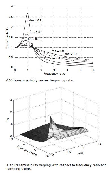
Figures 4.16 and 4.17 show the
variation of TR for various values of frequency ratios for different values of
damping.
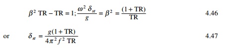
Effectiveness of foundation
For the design of a vibration isolation system, it is
convenient to express behaviour of the system in terms of isolation
effectiveness rather than transmissibility effectiveness. An isolation system
(see Fig. 4.15) is effective only if ╬▓ > 1.414 and since damping is undesirable in that range, it
is evident
that isolated monitoring should
have very little damping. When Žü = 0 and ╬▓ >
1.414 TR = 1/(╬▓2 ŌĆ' 1).
Then in that case effectiveness of the foundation is given by (1ŌĆ'TR).
Simplifying we get
Displacement
isolation
Consider the spring mass damper system shown in Fig. 4.18 in
which the support moves by xs. The equation of motion is
written as
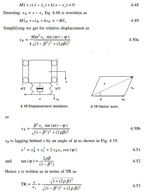
Hence transmissibility of force and displacement are the same.
Vibration-measuring
instruments
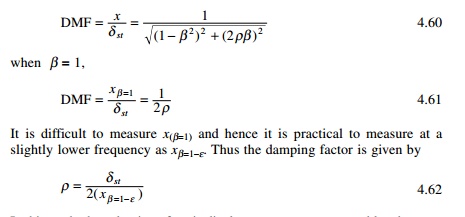
ŌĆó Seismometer:
This
works for large values of ╬▓ or a low value of natural frequency.
Hence a seismometer is a low natural frequency instrument. When ╬▓ becomes infinity, the relative
displacement xR becomes equal to xs (see Eq.
4.50a). The mass M then remains stationary while the supporting case
moves with the vibrating body. A large seismometer is required.
This instrument will have natural frequency of 2ŌĆ'5 Hz and a
useful range of 10ŌĆ'500Hz.
Accelerometer: These instruments are of
smaller size with high sensitivity. Using the instrument acceleration is
obtained and velocity and displacement are obtained by integration. Examining
Eq. 4.50a when ╬▓ Ōå' 0
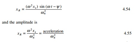
Accelerometers are high-frequency
instruments and the useful range for ╬▓ is from zero to 0.4. Those used for earthquake measurements
have a natural frequency of 20 Hz, which allows ground motion of frequency less
than 8Hz to be reproduced. This is shown in Fig. 4.20.
How to evaluate
damping in SDOF
1 Amplitude
decrement in free vibration
We have seen in last Session (Pages) that logarithmic
decrement is written as
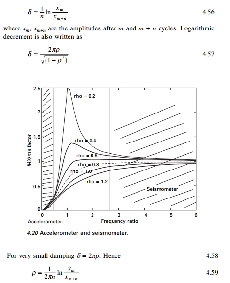
By using a minimal
instrumentation, one can find the damping coefficient by measuring amplitudes
at m and m + n cycles.
2 Measuring
resonant amplitude
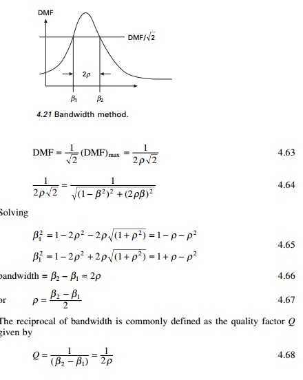
Harmonic excitation is applied to the structure by applying
harmonic load F0 sin (Žēt). A frequencyŌĆ'response curve for
a damped structure is shown in Fig. 4.7. The dynamic magnification factor
(DMF) is given by
In this method, evaluation of
static displacement may pose a problem because many type of loading systems
cannot be operated at zero frequency.
3 Bandwidth
methods (see Fig. 4.21)
To determine the damping factor
by this method determine the frequency ratio ╬▓ for which
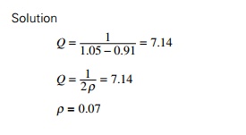
Example 4.11
Data collected from a frequency response test of a structure were plotted to construct a response curve similar to the one shown for DMF vs. frequency ratio. From the plot it was determined that DMFmax was 1.35 and DMF at half power points was 0.95. The response ratios corresponding to half power points are 0.91 and 1.05 respectively. Estimate the amount of damping in the system.
Response to ground
acceleration
Referring to Fig. 4.15 when the base moves by xg
the equation of motion is written as
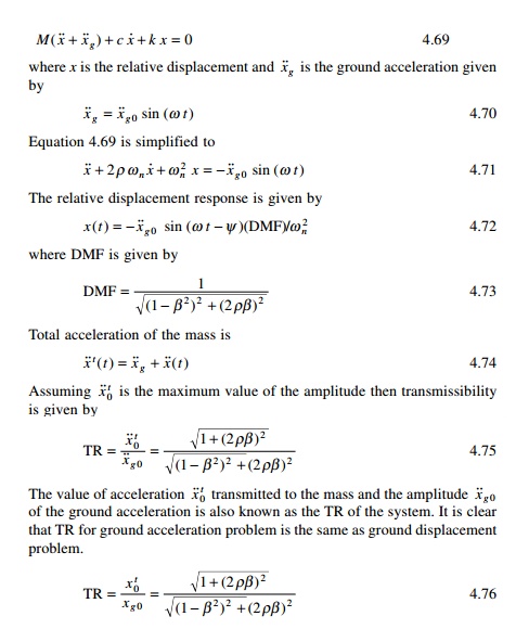
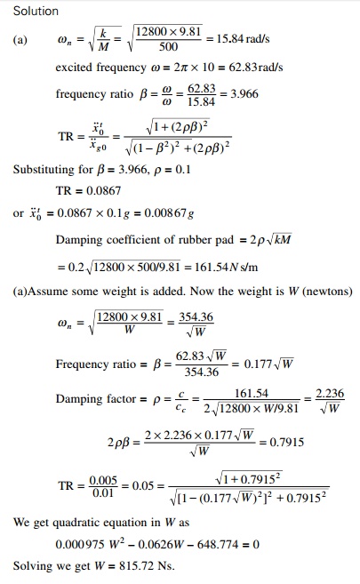
Example 4.12
A sensitive instrument with
weight 500N is to be installed at a location where vertical acceleration is 0.1g
and at frequency = 10Hz. This instrument is mounted on a rubber pad of
stiffness 12800 N/m and damping such that the damping factor is 0.1.
(a) What
acceleration is transmitted to the instrument?
If the instrument can tolerate only an acceleration of 0.005
suggest a solution assuming that the same rubber pad is used.
Related Topics