Chapter: Civil : Structural dynamics of earthquake engineering
Response to base excitation
Response to base
excitation
Evaluating the dynamic response of structures due to arbitrary
base or support motion can generally be facilitated by numerical
integration methods. The response of structures to base excitation is
the most important consideration in earthquake engineering. Consider the one
storey shear frame shown in Fig. 7.13. The structure experiences any arbitrary
ground displacements or acceleration u˙˙g ( t
). It is assumed that the shear frame is attached to a rigid base that moves
with the ground. In analysing the structural response there are several
components of motion that must be considered; specifically ui.
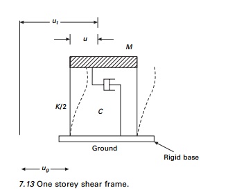
The relative displacement of the structure and uT
the total or absolute displacement of the structure measured from reference
axis.

The zero on the right hand side
of Eq. 7.61 would suggest that the structure is not subjected to any external
load F(t). This is not entirely true since the ground motion
creates the inertia of forces in the structure.
Thus, noting total displacement of the mass ut
is given by
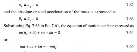
The term mu˙˙g can be thought
of as an effective load Feff (t) applied externally in
the mass of the structure shown in Fig. 7.14. Therefore the equation of motion
Note that in Eq. 7.69. u i
, u˙ i , u˙˙i
represent relative displacement, velocity and acceleration of the mass
respectively. We will see in later chapters that we can convert an ŌĆśnŌĆÖ-degrees-of-freedom
system to ŌĆśn-single-degree-of-freedom systemŌĆÖ for linear vibration with
proportional damping.
Equation 7.69 can be integrated
by any of the methods discussed in the chapter. We will apply the Wilson-╬Ė method. This is also useful in
establishing response spectra.
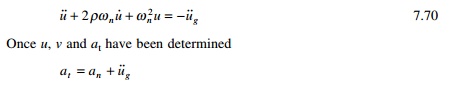
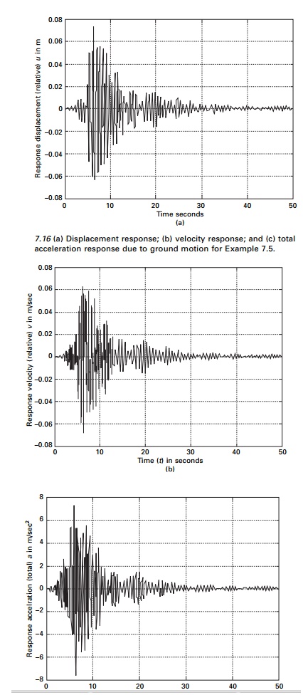
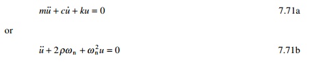
Example 7.5
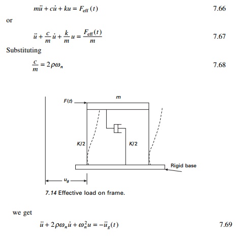
A single storey shear frame shown in Fig 7.15a is subjected to
El Centro ground excitation as shown in Fig. 7.15c. The simplified model is
shown in
Fig. 7.15b. The rigid girders
support a load of 25.57kN/m. Assuming a damping factor Žü = 0.02 for steel frame, E
= 200GPa. Write a computer program for the Wilson-╬Ė method to evaluate dynamic
response of the frame and plot u(t), v(t) and at(t)
in the interval.
Solution
Žēn =
9.53rad/s
Tn
=
0.659s
Žü = 0.02
The absolute acceleration can be obtained. The program using
Wilson-╬Ė method is given below for ground movement.
The displacement, velocity and acceleration (total) response are shown in Fig
7.16.
Program 7.8: MATLAB program for dynamic response to base
excitation using Wilson-╬Ė
method
% Response due
to ground excitation using Wilson-Theta method
%**********************************************************
ma=1;
k=90.829;
wn=sqrt(k/ma);
tn=6.283/wn;
theta=1.42;
r=0.02;
c=2.0*r*sqrt(k*ma);
u(1)=0;
v(1)=0;
tt=50.0;
n=2500;
n1=n+1;
dt=tt/n;
d=xlsread(ŌĆśeqdataŌĆÖ);
for i=1:n1;
ug(i)=d(i,2);
p(i)=-ug(i)*9.81;
end;
an(1)=(p(1)-c*v(1)-k*u(1))/ma;
kh=k+3.0*c/(theta*dt)+6.0*ma/(theta*dt)^2;
a=6.0*ma/(theta*dt)+3.0*c;
b=3.0*ma+theta*dt*c/2.0;
for i=1:n1;
s(i)=(i-1)*dt;
end;
for i=2:n1;
ww=(p(i)-p(i-1))*theta+a*v(i-1)+b*an(i-1);
xx=ww/kh;
zz=(6.0*xx/((theta*dt)^2)-6.0*v(i-1)/(theta*dt)-3.0*an(i-1))/theta;
yy=dt*an(i-1)+dt*zz/2.0;
v(i)=v(i-1)+yy;
an(i)=an(i-1)+zz;
vv=dt*v(i-1)+dt*dt*(3.0*an(i-1)+zz)/6.0;
u(i)=u(i-1)+vv;
end;
% Find total
acceleration
for i=1:n1;
an(i)=an(i)+ug(i)*9.81;
end;
figure(1);
plot(s,u);
xlabel(ŌĆś
time (t) in secondsŌĆÖ);
ylabel(ŌĆś Response displacement (relative) u in mŌĆÖ); title(ŌĆś
dynamic responseŌĆÖ);
figure(2);
plot(s,v);
xlabel(ŌĆś
time (t) in secondsŌĆÖ);
ylabel(ŌĆś Response velocity (relative) v in m/secŌĆÖ); title(ŌĆś
dynamic responseŌĆÖ);
figure(3);
plot(s,an);
xlabel(ŌĆś
time (t) in secondsŌĆÖ);
ylabel(ŌĆś Response acceleration (total) a in m/secŌĆÖ); title(ŌĆś
dynamic responseŌĆÖ);
figure(4);
plot(s,ug);
xlabel(ŌĆś time (t) in secondsŌĆÖ);
ylabel(ŌĆś ground acceleration / gŌĆÖ); title(ŌĆś Elcentro NSŌĆÖ);
WilsonŌĆÖs procedure
(recommended)
Damped free vibration due to
initial conditions
The equation of motion is written as
in which initial nodal
displacements u0 and velocity u˙0
are specified due to previous loading acting on the structure. Note that the
functions s(t) and c(t) given in Table 7.13 are
solutions to Eq. 7.71a.
There are many different methods
available to solve the typical modal equations. However, according to Wilson,
the use of the exact solutions for a linear load over a small time increment
has been found to be the most economical and accurate method to numerically
solve the equations using a computer program. This method does not have
problems such as stability and does not introduce numerical damping. Since the
most seismic ground motion is defined a linear within 0.005s intervals, the
method is exact for the type of loading for all frequencies. All modal
equations are converted to ŌĆśnŌĆÖ uncoupled equations.
Using the equation as
where time ŌĆśtŌĆÖ refers to the start of time step. Now
the exact solution within the time step can be written as

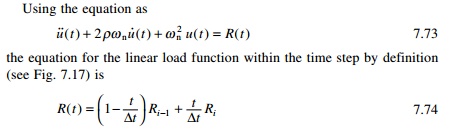
where all functions are as defined in Table 7.14.
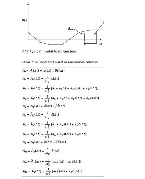
Equations 7.75, 7.76a and 7.76b are evaluated at the end of
time increment Ōłåt and the
following displacement, velocity and acceleration at the end of ith time
step are given by the recurrence relation.
The constants A1 to A12
are summarized in Table 7.14 and they need to be calculated only once.
Therefore for each time increment only 12 multiplications and 9 conditions are
required. Hence the computer time required solving for 200 steps per second for
50s duration earthquake approximately 0.01s or 100 modal equations can be
solved in 1s of computer time. Therefore, there is no need to consider other
numerical methods (as per Wilson) such as approximate fast Fourier transform,
or numerically evolution of the Duhamel integral to solve the equation.
Because of the speed of this
exact piecewise linear technique, it can also be used to develop accurate
earthquake response spectra using a very small amount of computer time.
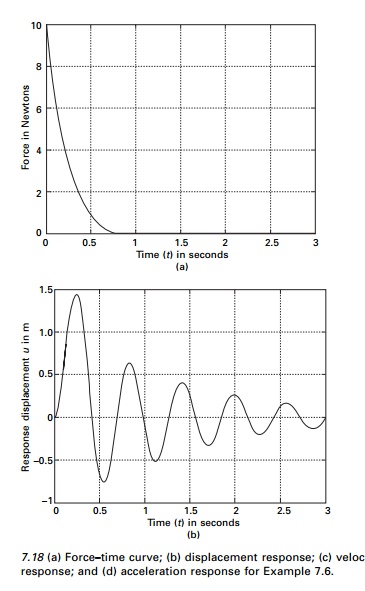
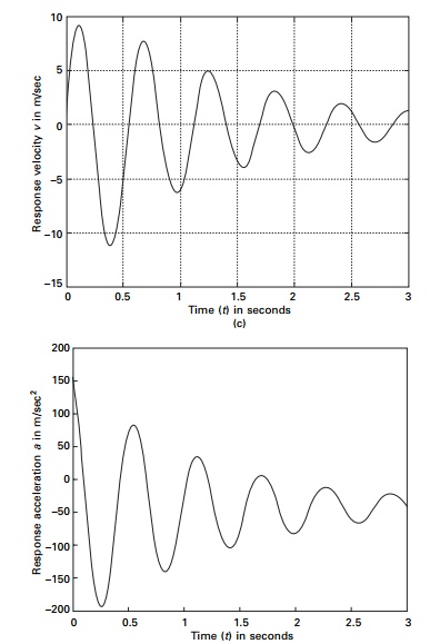
Example 7.6
Solve Example 7.4 by WilsonŌĆÖs
proposed procedure with different data as shown below.
m = 0.065 k = 7.738 Žü = 0.07 F0 =
10
Solution
The equation of motion is written as
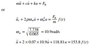
A program for WilsonŌĆÖs method is written in MATLAB as shown
below. The force time curves are shown in Fig. 7.18a. The displacement,
velocity and acceleration response are shown in Fig.7.18b, c and d
respectively. WilsonŌĆÖs method is the best to solve problems involving base excitation.
Program 7.9: MATLAB program
for dynamic response by WilsonŌĆÖs general method
%Matlab program using WilsonŌĆÖs
general method %********************************************* ma=0.065;
k=7.738;
wn=sqrt(k/ma)
r=0.07; wd=wn*sqrt(1-r^2); c=2.0*r*sqrt(k*ma); wnb=wn*r;
rb=r/sqrt(1-r^2); tt=3.0;
n=300
n1=n+1
dt=tt/n
td=.75;
jk=td/dt;
a0=2.0*r/(wn*dt);
a1=1+a0 a2=-1/dt;
a3=-rb*a1-a2/wd; a4=-a1;
a5=-a0; a6=-a2;
a7=-rb*a5-a6/wd; a8=-a5;
a9=wd^2-wn^2; a10=2.0*wnb*wd; u(1)=0;
v(1)=0;
for m=1:n1; pa(n)=0.0 p(m)=0.0;
end;
jk1=jk+1; for n=1:jk1;
t=(n-1)*dt;
p(n)=10.0*(1-t/td)*exp(-2.0*t/td);
p(n)=pa(n)/ma;
end; s=exp(-r*wn*dt)*sin(wd*dt);
c=exp(-r*wn*dt)*cos(wd*dt); sd=-wnb*s+wd*c; cd=-wnb*c-wd*s; sdd=-a9*s-a10*c cdd=-a9*c+a10*s;
ca1=c+rb*s;
ca2=s/wd;
ca3=(a1+a2*dt+a3*s+a4*c)/(wn^2);
ca4=(a5+a6*dt+a7*s+a8*c)/(wn^2)
ca5=cd+rb*sd;
ca6=sd/wd;
ca7=(a2+a3*sd+a4*cd)/(wn^2);
ca8=(a6+a7*sd+a8*cd)/(wn^2);
ca9=cdd+rb*sdd;
ca10=sdd/wd;
ca11=(a3*sdd+a4*cdd)/(wn^2);
ca12=(a7*sdd+a8*cdd)/(wn^2);
an(1)=(p(1)-2.0*r*wn*v(1)-(wn^2)*u(1)); for i=1:n1
ti(i)=(i-1)*dt end
for i=2:n1
u(i)=ca1*u(i-1)+ca2*v(i-1)+ca3*p(i-1)+ca4*p(i);
v(i)=ca5*u(i-1)+ca6*v(i-1)+ca7*p(i-1)+ca8*p(i);
an(i)=an(i-1)+ca9*u(i-1)+ca10*v(i-1)+ca11*p(i-1)+ca12*p(i);
end;
figure(1);
plot(ti,u);
xlabel(ŌĆś
time (t) in secondsŌĆÖ)
ylabel(ŌĆś Response displacement u in mŌĆÖ) title(ŌĆś dynamic
responseŌĆÖ)
figure(2);
plot(ti,v);
xlabel(ŌĆś
time (t) in secondsŌĆÖ)
ylabel(ŌĆś Response velocity v in m/secŌĆÖ) title(ŌĆś dynamic
responseŌĆÖ)
figure(3);
plot(ti,an);
xlabel(ŌĆś
time (t) in secondsŌĆÖ)
ylabel(ŌĆś Response acceleration a in m/secŌĆÖ) title(ŌĆś dynamic
responseŌĆÖ)
figure(4);
plot(ti,p)
xlabel(ŌĆś time (t) in secondsŌĆÖ)
ylabel(ŌĆś force in NewtonsŌĆÖ) title(ŌĆś Excitation ForceŌĆÖ)
Response of
elasto-plastic SDOF system
When a steel or reinforced
concrete building is subjected to extreme loading it undergoes elasto-plastic
behaviour. Usually excursions beyond the elastic range are not permitted under normal
conditions of operation; the extent of the permanent damage the structure may
sustain when subjected to extreme conditions such as blast or earthquake
loading is frequently of interest to the design engineer.
Consider a one storey structural steel shear frame subjected
to a horizontal static force F as shown in Fig. 7.19. Assume the girder
to be infinitely rigid
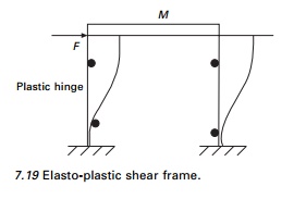
compared with the column, when
the load is applied numerically with the frame. Plastic hinges will eventually
form at the end of the columns. The plot of resistance versus displacement
relationship is given in Fig. 7.20a. The behaviour is linear up to the point ŌĆśaŌĆÖ
corresponding to resistance Ry where first yielding in the
cross section occurs. As the load is increased, the resistance curve becomes
nonlinear as the column cross-sections plasticize under the system softens. The
full plastification of the cross-section occurs at point ŌĆśbŌĆÖ
corresponding to maximum resistance Rm. Upon unloading, the
system rebounds elastically along the line ŌĆśbcŌĆÖ parallel to initial
linear portion ŌĆśOaŌĆÖ. The system remains elastic until first yielding
again attained at point ŌĆśdŌĆÖ corresponding to resistance Ry.
As the load is increased, further plastic hinges reform at - Rn
corresponding to point ŌĆśeŌĆÖ. Unloading will be linear elastic parallel to
line ŌĆścdŌĆÖ.
If the maximum positive and
negative resisting forces Rm and -Rm are
numerically equal, the hysteresis loop formula by the cyclic loading will be
symmetric with respect to origin. For each cycle, energy is dissipated by an
amount that is proportional to the area within the hysteresis loop. The
behaviour illustrated in Fig. 7.20a is often simplified by assuming linear
behaviour up to the point of plastification. This type of behaviour is referred
to as ŌĆśelasto-plasticŌĆÖ. This slope of the elastic loading and unloading
curve is proportional to stiffness. The elasto-plastic behaviour can be
idealized shown in Fig 7.20b. One hysteresis loop is discussed below.
Stage 1 Elastic loading
This is defined by segment ŌĆśoaŌĆÖ
on the resistance displacement curve 0 Ōēż
u Ōēż uel and u╦Ö
> 0 where uel = Rm/k.
The resisting force as the stages is given by
Rm = Kx -- - - - - -7.78
Unloading in the stage occurs when u˙ < 0.
Stage 2 Plastic loading
This stage is represented by the segment ab on the
resistance-displacement
curve and corresponds to the
condition uel < u <umax and u˙
> 0 where u max is the displacement in hysteresis loop.
The resisting force in this stage is
given by
Fs = Rm - -- - - - - -7.79
Stage 3 Elastic rebound
This stage is defined by the segment bc on the
resistance-displacement
curve and corresponds to a condition (umax-2
uel) < u < umax and u˙ <
0. The resistance is given by
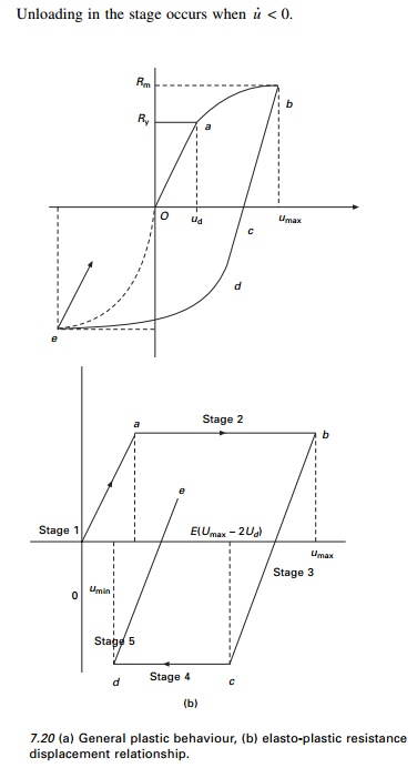
It is to be noted that load
reversal in this stage occurs than u < ( u
max Ōł' 2u╦Ö)
and u˙ < 0 .
Stage 4 Plastic loading
The system response in this stage
is represented by segment ŌĆścdŌĆÖ on the resistance displacement curve and
corresponds to condition umin < u < (umax
-uel) and u˙ < 0 where umin
is the minimum displacement as the stage. The system resistance is given by
Stage 5 Elastic rebound
Once the cycle of hysteresis is completed, the system unloads
elastically along segment ŌĆśdeŌĆÖ. This stage corresponds to the condition umin
< u < (umin + 2uel) and u˙
> 0. This resisting force is given by
Fs = k(u
- umin) - Rm -- 7.82
Program 7.10: MATLAB
program for dynamic response for elasto-plastic SDOF system
%program
for elasto-plastic analysis
%simulates nonlinear response of
SDOF using %elasto-plastic hysteresis loop to model
%spring resistance. The program
uses Newmark-B integration scheme clc;
k=1897251;
m=43848;
c=7767.7;
%for
elasto-plastic rm=66825.6 and
%for elastic response rm is
increased such that rm=6682500.6 rm=66825.6;
tend=30.0;
h=0.02;
nfor=1500;
%earthquake
data
%d=xlsread(ŌĆśeldatŌĆÖ);
%for
i=1:nfor
% tt(i)=d(i,1);
% ft(i)=d(i,2);
% ft(i)=m*ft(i)*9.81;
%end
%force data d=xlsread(ŌĆśforcedatŌĆÖ)
for i=1:nfor
tt(i)=d(i,1)
ft(i)=d(i,2) end
ic=1;
for t=0:h:tend for i=1:nfor-1
if (t >= tt(i)) & (t < tt(i+1))
p(ic)=ft(i)+(ft(i+1)-ft(i))*(t-tt(i))/(tt(i+1)-tt(i));
ic=ic+1; continue
end continue continue
end end x(1)=0; x1(1)=0;
x2(1)=p(1)/m;
xel=rm/k;
xlim=xel; xmin=-xel; a1=3/h; a2=6/h; a3=h/2; a4=6/(h^2);
kelas=k+a4*m+a1*c
kplas=a4*m+a1*c
ic=2;
loop=1;
for t=h:h:tend-30*h if loop==1
[x,x1]=Respond(kelas,p,x,x1,x2,m,c,ic,a2,a3,a1);
r=-rm-(xmin-x(ic))*k; x2(ic)=(p(ic)-c*x1(ic)-r)/m;
if x(ic) >= xlim loop=2;
end ic=ic+1; continue
elseif(loop==2)
loop;
[x,x1]=Respond(kplas,p,x,x1,x2,m,c,ic,a2,a3,a1);
r=rm; x2(ic)=(p(ic)-c*x1(ic)-r)/m; if x1(ic)<=0
loop=3;
xmax=x(ic); xlim=x(ic)-2*xel; end
ic=ic+1; continue elseif(loop==3)
loop;
[x,x1]=Respond(kelas,p,x,x1,x2,m,c,ic,a2,a3,a1);
r=rm-(xmax-x(ic))*k; x2(ic)=(p(ic)-c*x1(ic)-r)/m;
if x(ic)<=xlim loop=4;
end ic=ic+1;
continue elseif(loop==4)
loop;
[x,x1]=Respond(kplas,p,x,x1,x2,m,c,ic,a2,a3,a1); r=-rm;
x2(ic)=(p(ic)-c*x1(ic)-r)/m; if x1(ic)>=0
loop=1
xlim=x(ic)+2.0*xel;
xmin=x(ic); end ic=ic+1;
continue end
end ic=ic-1; for i=1:ic
tx(i)=(i-1)*h; xx(i)=x(i);
end plot(tx,xx) hold on xlabel(ŌĆś
timeŌĆÖ)
ylabel(ŌĆś displacement in mŌĆÖ)
title(ŌĆś Displacement response history ŌĆś)
function
[x,x1]=Respond(k,p,x,x1,x2,m,c,ic,a2,a3,a1)
dps=p(ic)-p(ic-1)+x1(ic-1)*(a2*m+3*c)+x2(ic-1)*(3*m+a3*c); dx=dps/k;
dx1=a1*dx-3*x1(ic-1)-a3*x2(ic-1);
x(ic)=x(ic-1)+dx; x1(ic)=x1(ic-1)+dx1;
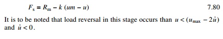
Example 7.7
A shear frame structure shown in
Fig. 7.4a is subjected to time varying force shown in Fig. 7.21. Evaluate the
elastic and elasto-plastic response of the structure by the Newmark method
without equilibrium iterations.
Solution
k =
1897251N/m
m = 43848kg
c = 34605.4Ns/m
Rm =
66825.6N
Ōłåt = 0.001
Figure 7.22 shows the
displacement due to loading for elastic and elasto-plastic cases.
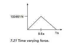
Response spectra by
numerical integration
Construction of response spectrum by analytical evaluation of
the Duhamel integral is quite tedious. To develop response spectrum by
numerical integration,
consider a family of SDOF oscillations shown in Fig. 7.23.
Each oscillator has different natural period and frequency:
T1< T2 < T3├ē├ēTn 7.83
Specify a function F(t).
The dynamic magnification factor can be calculated as

Finally DMF is plotted against desired spectrum curve.
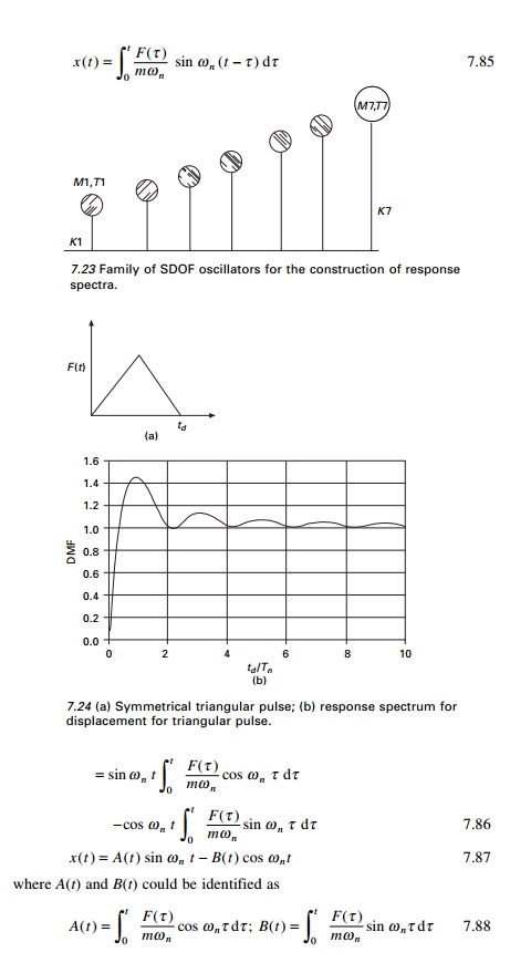
Example 7.8
Construct a response spectrum for
the symmetric triangle shown in Fig. 7.24a. Plot DMF vs td/T in
the integral 0 Ōēż td/T
Ōēż 10. Assume Žü = 0, td = 2s. A MATLAB program for drawing response
spectrum is given in Chapter 6. The response curve is shown in Fig. 7.24b.
Solution
A family of response spectrum curves or response spectra can
be produced for a specific load case by evaluating response maxima for several
values of damping Žü. Hence
maximum response of a linear SDOF to a specified time depends on Žēn and Žü.
Numerical method for
evaluation of the Duhamel integral
1.For an undamped system
The response of an undamped SDOF system subjected to a general
type of forcing function as given by the Duhamel integral as
The variation of displacement
with time is of interest. Time is divided into a number of equal intervals.
Each duration can be taken as Ōłåt and the
response at these sequences of time can be evaluated.
Applying SimpsonŌĆÖs rule
A(t -
2Ōłåt) is the
value of the integral at time instant (t - 2Ōłåt) by
summation of previous values. B(t) can be obtained in a
similar way.
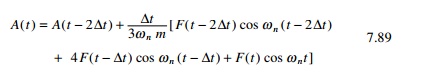
Example 7.9
A water tank shown in Fig. 7.25a
is subjected to a dynamic load shown in Fig. 7.25b. Evaluate numerically using
the Duhamel integral for the response.
Solution
mass = 400 ├-
1000/9.81 = 40774.7kg k = 35000 ├- 1000N/m
The values of A and B are evaluated as shown in
Table 7.15.
2.For an under-damped system
Again numerical integration by
SimpsonŌĆÖs rule can be carried out to find the values of A(t) and B(t)
and hence u(t).
Selection of direct
integration method
It is apparent that a large
number of different numerical integration methods are possible by specifying
different integration parameters. A few of the most commonly used methods are
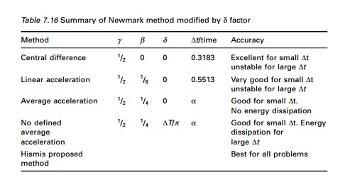
summarized in Table 7.16.
For SDOF systems the central
difference method is most accurate, and the linear acceleration method is more
accurate than the average acceleration method. It appears that the modified
average acceleration method, with a minimum addition of proportional damping is
a general procedure that can be used for the dynamic analysis of all structural
systems.
The basic Newmark constant
acceleration method can be extend to nonlinear dynamic analysis. This requires
that iterations must be performed at each time step in order to satisfy
equilibrium. For multiple degrees of freedom, which will be seen in later
chapters incremental matrix must be formed and triangularized at each iteration
or at selective point of time. Many different numerical tricks including
element by element methods have been developed in order to minimize
computational requirements.
Table 7.16 Summary of Newmark
method modified by ╬┤ factor
Summary
For earthquake analysis of linear
structures it should be noted that direct integration of the dynamic
equilibrium is normally not numerically efficient as compared to mode
superposition method (for MDOF). The Newmark constant acceleration method with
the addition of very small amount of stiffness proportional damping is
recommended for dynamic analysis of nonlinear structure systems.
In the area of nonlinear dynamic
analysis one cannot prove that any one method will always converge. One should
always check the error in the conservation of energy for every solution
obtained.
Related Topics