Chapter: Civil : Structural dynamics of earthquake engineering
Differential quadrature and transformation methods for vibration problems
Differential
quadrature and transformation methods for vibration problems in relation to
structural dynamics during earthquakes
Abstract: In this
page, natural frequencies are obtained for beam-like structures with
different boundary conditions using the differential quadrature method and
differential transformation methods. The results obtained are compared with
those obtained from the finite element method and other numerical methods.
Programs in MATLAB are given for solving beam problems by the differential
quadrature method. The symbolic programming package MATHEMATICA is ideally
suited to solve recursive equations of differential transformation methods.
Key words: differential quadrature, harmonic
quadrature, Lagrange interpolation, differential transformation,
boundary conditions, natural frequency.
Introduction
Numerical solutions to free
vibration analysis of beams and columns are obtained by the method of differential
quadrature (DQ) and harmonic differential quadrature (HDQ) for various
support conditions. The obtained results are compared with the existing
solutions available from other numerical methods such as finite element method
(FEM) and analytical results. In addition, this chapter also uses a recently
developed technique, known as the differential transformation (DT) to
determine the natural frequency of beams and columns. In solving the
problem, governing differential equations are converted to algebraic equations
using DT methods which must be solved together with applied boundary
conditions. The symbolic programming package MATHEMATICA is ideally suited to
solve such recursive equations by considering fairly large numbers of terms.
DQ method
These problems of free vibration
of beams and columns either prismatic or non-prismatic, could easily be solved
using the DQ method, which was introduced by Bellman and Casti (1971). With the
application of boundary conditions as per WilsonŌĆÖs method (Wilson 2002) the DQM
method will also be straightforward and easy for engineers to use. Since the
introduction of this method, applications of the DQ method to various
engineering problems have been investigated and their success has shown the
potential of the method as an attractive numerical analysis tool. The basic
idea of the DQM method is to quickly compute the derivatives of a function at
any grid point within its bounded domain by estimating the weighted sum of the
values of the functions at a small set of points related to the domain. In the
originally derived DQM, Lagrangian interpolation polynomial was used (Bert and
Malik 1996, Bert et al. 1993, 1994). A recent approach of the original
differential quadrature approximation, HDQ, was originally proposed by Striz et
al. (1995). Unlike the DQ method, HDQM uses harmonic or trigonometric
functions as the test functions. As the name of the test function suggested,
this is called the HDQ method. All the problems in this chapter have
demonstrated that the application of the DQ and HDQ methods will lead to
accurate results with less computational effort and that there is a potential
that the method may become alternative to conventional methods such as finite
difference, finite element and boundary element.
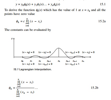
Lagrangian interpolation
This interpolation technique is applied if the given points may or may not be equally spaced (see Fig. 15.1). The polynomial is an approximation to the function f (x), which coincides with the polynomial at (xi, yi).
Differential quadrature
method formulation
The fourth order governing differential equation for free vibration of column with varying flexural rigidity ŌĆśDŌĆÖ (D = EI) and w (= the lateral deflection) may be written as
and the number of sampling points n > m.
A natural and often convenient choice for sampling point is
that of equally spaced points or CGL mesh distribution as given by Eq. 15.8.
For the sampling points, we adopt well accepted ChebyshevŌĆ'GaussŌĆ'Lobatto mesh
distribution given by Shu (2000) as
ŌĆśLŌĆÖ is the length of the
column, the column is divided into ŌĆśneŌĆÖ (say 40) divisions or ne+1
(41) sampling points in the case of DQM and xi is the
distance from the bottom end of the column.
HDQ method
The harmonic test function hi(╬Š) used in the HDQ method is
defined as
Higher order derivatives can be obtained using Eq. 15.9.
Transverse vibration of
pre-tensioned cable
The transverse vibration of a taut cable or string has an
equation of motion similar to the governing longitudinal vibration of a uniform
rod. Consider a uniform elastic cable, having mass/unit length (Žü A), Žü being the mass density, to be
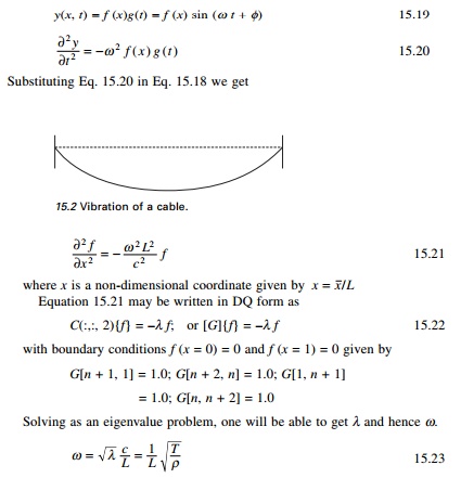
stretched under tension T between two fixed points as shown in Fig.
15.2. Assuming small deflections and slopes, the equation of motion for
transverse vibration is given by
where c = T/ŽüA is the
velocity of wave propagation along the cable and y is the transverse deflection
of the string at any distance x. The above equation is also identical to the
wave equation. The transverse deflection may be assumed as
A MATLAB program to find the
natural frequency of transverse vibration of pretensioned string is shown
below.
Program 15.1: MATLAB program
for finding the natural frequency of lateral vibration of pre-tensioned string
STRINGVIB
% free vibration of a
pretensioned cable by differential quadrature clc; close all;
ne=20;
n=ne+1;
nn=2*n;
no=4;
m=zeros(n,1);
x=zeros(n,1);
c=zeros(n,n,no);
d=zeros(n+2,n+2);
f=zeros(n+2,n+2);
%give length and mass density and
area of the cable l=1;
dl=l/ne;
rho=7800;
ar=0.005;
ma=rho*ar;
%give tension in the cable
T=4*ma;
format long; for i=1:n
x(i)=.5*(1-cos((i-1)*pi/ne)); end
%c=qquadrature(x,n,no);
c=harquadrature(x,n,no);
d(1:n,1:n)=c(:,:,2)/l^2;
%application of boundary
conditions d(n+1,1)=1.0;
d(n+2,n)=1.0;
d(1,n+1)=1.0;
d(n,n+2)=1.0;
din=inv(d); f(1:n,1:n)=-eye(n,n);
ddf=din*f; [u,eu]=eig(ddf);
for i=1:n ww1(i)=u(i,3); ww2(i)=u(i,4);
ww3(i)=u(i,5);
end
disp(ŌĆś fundamental natural
frequency\nŌĆÖ) wn1=sqrt(T/(eu(3,3)*ma)) disp(ŌĆśfundamental mode shape\nŌĆÖ)
ww1'
disp(ŌĆś second natural frequencyŌĆÖ)
wn2=sqrt(T/(eu(4,4)*ma)) disp(ŌĆśsecond mode shapeŌĆÖ)
ww2'
disp(ŌĆś third natural frequencyŌĆÖ)
wn3=sqrt(T/(eu(5,5)*ma)) disp(ŌĆś third mode shapeŌĆÖ) ww3'
figure(1);
plot(x,ww1);
xlabel(ŌĆśxŌĆÖ);
ylabel(ŌĆśwŌĆÖ);
title(ŌĆś fundamental mode shapeŌĆÖ);
figure(2);
plot(x,ww2);
xlabel(ŌĆśxŌĆÖ);
ylabel(ŌĆśwŌĆÖ);
title(ŌĆś fundamental mode shapeŌĆÖ);
figure(3);
plot(x,ww3);
xlabel(ŌĆśxŌĆÖ);
ylabel(ŌĆśwŌĆÖ);
title(ŌĆś fundamental mode shapeŌĆÖ);
function[y]=harquadrature(x,n,no)
m=zeros(n,1);
c=zeros(n,n,4); for i=1:n
m(i,1)=1; for k=1:n
if ((k ==i )) jk=i;
else m(i,1)=m(i,1)*sin((x(i)-x(k))*pi/2);
format long end
end end m;
for i=1:n for j=1:n
if(j==i)
jk=i; else
c(i,j,1)=(pi*m(i,1))/(2.0*sin((x(i)-x(j))*pi/2)*m(j,1));
end
end end
for i=1:n c(i,i,1)=0.0;
for j=1:n if ((i==j)) jk=i;
else c(i,i,1)=c(i,i,1)-c(i,j,1);
end
end end o=2;
for i=1:n for j=1:n
if(j==i)
jk=i; else
c(i,j,o)=c(i,j,1)*(2.0*c(i,i,1)-pi/tan(((x(i)-x(j))*pi/2)));
end
end end
for i=1:n c(i,i,2)=0.0;
for j=1:n if ((i==j)) jk=i;
else c(i,i,2)=c(i,i,2)-c(i,j,2);
end
end end
for o=3:no for i=1:n
for j=1:n c(i,j,o)=0.0;
for k=1:n c(i,j,o)=c(i,j,o)+c(i,k,1)*c(k,j,(o-1));
end end
end end y=c;
function[y]=qquadrature(x,n,no)
m=zeros(n,1);
c=zeros(n,n,4); for i=1:n
m(i,1)=1; for k=1:n
if ((k ==i )) jk=i;
else m(i,1)=m(i,1)*(x(i)-x(k));
format long end
end end
for i=1:n for j=1:n
if(j==i)
jk=i; else
c(i,j,1)=m(i,1)/((x(i)-x(j))*m(j,1)); end
end end
for i=1:n c(i,i,1)=0.0;
for j=1:n if ((i==j)) jk=i;
else c(i,i,1)=c(i,i,1)-c(i,j,1);
end
end end
for o=2:no for i=1:n
for j=1:n c(i,j,o)=0.0;
for k=1:n c(i,j,o)=c(i,j,o)+c(i,k,1)*c(k,j,(o-1));
end end end
end c(:,:,1); y=c;
OUTPUT
fundamental natural frequency
wn1 = 6.28318530717963
fundamental mode shape ans =
0
0.00733128915883
0.02911774918179
0.06459034487273
0.11203447410058
0.16833305876402
0.22868163719304
0.28673229986014
0.33532231670280
0.36772667715649
0.37911498526798
0.36772667715649
0.33532231670280
0.28673229986015
0.22868163719305
0.16833305876402
0.11203447410058
0.06459034487273
0.02911774918180
0.00733128915883
0
second natural frequency wn2 =
12.56637061435911
second mode shape
ans =
0
0.01384802941406
0.05484814152807
0.12024309852971
0.20220761642762
0.28495445387276
0.34458819094757
0.35438646074539
0.29557188373010
0.16900007820430
-0.00000000000001
-0.16900007820432
-0.29557188373010
-0.35438646074539
-0.34458819094755 -0.28495445387275 -0.20220761642761
-0.12024309852971 -0.05484814152806 -0.01384802941406 0
third natural frequency wn3 =
18.84955592153890 third mode shape
ans =
0
0.02026414001026
0.07989008567297
0.17170783853740
0.27374891998932
0.34314670851919
0.32560576874274
0.18817009067074 -0.03995789607568 -0.25873859745335
-0.34947339621276 -0.25873859745337 -0.03995789607570 0.18817009067073
0.32560576874275 0.34314670851920 0.27374891998931 0.17170783853740
0.07989008567298 0.02026414001026 0
Example 15.1
A string of length 1 m subjected to pre-tension of 156 N is
under transverse vibration. Calculate the first three fundamental natural
frequencies assuming mass density = 7800 kg/m3 and area of the cable
= 0.005 m2.
Solution
The nth natural frequency is given by
Žēn = 2 n
ŽĆ
Žē1 = 6.2831
rad/s; Žē2 = 12.566
rad/s; Žē3 =
18.8493 rad/s
The values obtained by DQ are
Žē1 = 6.2831
rad/s; Žē2 =
12.5633 rad/s; Žē3 =
18.8495 rad/s
which agree with the true values.
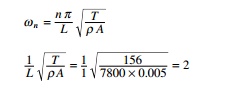
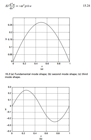
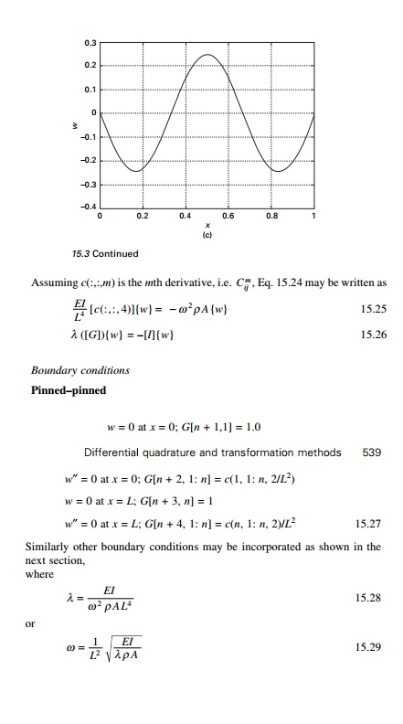
The mode shapes corresponding to these three frequencies are shown in Fig. 15.3
for first, second and third modes.
Lateral vibration of uniform
Euler beams
The governing differential equation of lateral vibration of
uniform beams is given as
Example 15.2
Find the fundamental three
natural frequencies of a simply supported beam given that E = 200 GPa; I
= 18.6 ├- 10ŌĆ'6; A = 2.42 ├- 10ŌĆ'4; Žü = 7800 kg/m3;
L = 20 m.
Solution
The closed form solutions for the problem are given by
Program 15.2: MATLAB program
for free vibration of an Euler beam
EULERBEAMVIB
% free vibration of a beam by
differential quadrature for different boundary conditions
clc; close all; ne=20; n=ne+1;
nn=2*n; no=4; m=zeros(n,1); x=zeros(n,1);
c=zeros(n,n,no);
d=zeros(n+4,n+4);
f=zeros(n+4,n+4); iy=18.6e-6;
ar=2.42e-4; ymod=200e9; l=20.0;
dl=l/ne;
mden=7800; format long; for i=1:n
x(i)=.5*(1-cos((i-1)*pi/ne)); end
c=qquadrature(x,n,no);
%c=harquadrature(x,n,no);
d(1:n,1:n)=ymod*iy*c(:,:,4)/l^4;
%application of boundary conditions %pinned - pinned
d(n+1,1)=1.0;
d(n+2:n+2,1:n)=c(1,1:n,2)/l^2;
d(n+3,n)=1.0;
d(n+4:n+4,1:n)=c(n,1:n,2)/l^2;
d(1,n+1)=1.0;
d(n,n+3)=1.0; for i=1:n
d(i,n+2)=d(n+2,i);
d(i,n+4)=d(n+4,i); end
%fixed ŌĆ' fixed
%d(n+1,1)=1.0;
%d(n+2:n+2,1:n)=c(1,1:n,1)/l;
%d(n+3,n)=1.0
%d(n+4:n+4,1:n)=c(n,1:n,1)/l;
%d(1,n+1)=1.0;
%d(n,n+3)=1.0;
%for i=1:n
%d(i,n+2)=d(n+2,i);
%d(i,n+4)=d(n+4,i);
%end
%fixed - free
%d(n+1,1)=1;
%d(n+2:n+2,1:n)=c(1,1:n,1)/l;
%d(n+3:n+3,1:n)=c(n,1:n,2)/l^2;
%d(n+4:n+4,1:n)=c(n,1:n,3)/l^3;
%for i=1:n
%d(i,n+1)=d(n+1,i);
%d(i,n+2)=d(n+2,i);
%d(i,n+3)=d(n+3,i);
%d(i,n+4)=d(n+4,i);
%end
din=inv(d);
f(1:n,1:n)=eye(n,n);
ddf=din*f;
[u,eu]=eig(ddf); for i=1:n
ww1(i)=u(i,5);
ww2(i)=u(i,6);
ww3(i)=u(i,7); end
sprintf(ŌĆś fundamental natural
frequencies\nŌĆÖ) wn1=sqrt(1/(mden*ar*eu(5,5))) wn2=sqrt(1/(mden*ar*eu(6,6)))
wn3=sqrt(1/(mden*ar*eu(7,7)))
sprintf(ŌĆś fundamental mode
shape\nŌĆÖ) ww1'
figure(1);
plot(x,ww1);
xlabel(ŌĆśxŌĆÖ);
ylabel(ŌĆśwŌĆÖ);
title(ŌĆś fundamental mode shapeŌĆÖ);
figure(2);
plot(x,ww2);
xlabel(ŌĆśxŌĆÖ);
ylabel(ŌĆśwŌĆÖ);
title(ŌĆś second mode shapeŌĆÖ);
figure(3);
plot(x,ww3);
xlabel(ŌĆśxŌĆÖ);
ylabel(ŌĆśwŌĆÖ);
title(ŌĆś third mode shapeŌĆÖ);
OUTPUT
ans =
fundamental
natural frequencies
wn1 = 34.63827370993050
wn2 = 1.385530948382473e+002
wn3 = 3.117444633857984e+002
To find
natural frequency and mode shape given variation of D = EI for Euler beam with
axial load
In this problem, (D = EI) and P are known and w and Žē are
unknown values that can be found by solving as an eigenvalue problem as
explained below. Assuming c(:,:,m) is the mth derivative , i.e. C m , the governing equation may be
written as
Boundary conditions
Since it is a fourth order differential equation, four
boundary conditions should be given. The boundary conditions will be applied as
follows.
ClampedŌĆ'pinned
w = 0 at x = 0; G[n
+ 1, 1] = 1.0
wŌĆ▓ = 0 at x = 0; G[n + 2, 1:
n] = c(1, 1: n, 1)/L
w = 0 at x = L; G[n
+ 3, n] = 1
wŌĆ│ = 0 at x = L; G[n + 4,
1: n] = c(n, 1: n, 2)/L2 ----15.35
ClampedŌĆ'clamped
w = 0 at
x = 0; G[n + 1, 1] = 1.0
wŌĆ▓ = 0 at x = 0; G[n + 2, 1:
n] = c(1, 1: n, 1)/L w = 0 at x = L;
G[n + 3, n] = 1
wŌĆ▓ = 0 at
x = L; G[n + 4, 1: n] = c(n, 1:
n, 2)/L --- 15.36
PinnedŌĆ'pinned
w = 0 at
x = 0; G[n + 1, 1] = 1.0
wŌĆ│ = 0 at x = 0; G[n + 2, 1:
n] = c(1, 1: n, 2/L2) w = 0 at x =
L; G[n + 3, n] = 1
wŌĆ│ = 0 at
x = L; G[n + 4, 1: n] = c(n, 1:
n, 2)/L2 ---
15.37
ClampedŌĆ'free
w = 0 at
x = 0; G[n + 1, 1] = 1.0
wŌĆ▓ = 0 at x = 0; G[n + 2, 1:
n] = c(1, 1: n, 1)/L wŌĆ│ = 0 at x = L; G[n + 3,
n] = c(n, 1: n, 2)/L2
dD w ŌĆ▓ŌĆ▓ + Dw ŌĆ▓ŌĆ▓ŌĆ▓ = Ōł' Pw ŌĆ▓ at x = L ; G [n + 4,1: n] dx
= ╬▒nnc(n,
1: n, 2)/L2 + Dnnc(n, 1: n,
3)/L3
ŌĆ'Pc
(n, 1: n, 1)/L --- 15.38
1WilsonŌĆÖs method (Wilson, 2002) of applying
boundary conditions
In general, the boundary conditions are given by
[G]1{w}
= [E]1{w}
--- 15.39
Combining governing equations and boundary conditions, we get
The above equation has both
equilibrium and equation of geometry. Solving Eq. 15.41 is an eigenvalue
problem; one will be able to obtain the natural frequency.
Program 15.3: MATLAB program
for solving free vibration problem of non-prismatic beam with or without axial
load
EULERVIB
% free vibration of non-prismatic
Euler beams with or without axial load %using differential quadrature method
clc;
ne=50;
n=ne+1;
nn=2*n;
no=4;
m=zeros(n,1);
x=zeros(n,1);
xi=zeros(n,1);
c=zeros(n,n,no);
d=zeros(n+4,n+4);
e=zeros(n+4,n+4);
z=zeros(n+4,1);
f=zeros(n+4,1);
alp=zeros(n,n);
bet=zeros(n,n);
zz=zeros(n,1);
ki=zeros(n,n);
eta=zeros(n,n);
const=1.0;
l=12;
ymod=200e09;
rho=7800; format long; for i=1:n
xi(i)=.5*(1-cos((i-1)*pi/ne));
%mi(i)=0.000038*(1-xi(i)^2/2);
ar(i)=1/rho;
mi(i)=0.000038;
ki(i,i)=ymod*mi(i);
end
c=qquadrature(xi,n,no);
%c=harquadrature(xi,n,no)
for i=1:n
alp(i,i)=0;
bet(i,i)=0;
for j=1:n
alp(i,i)=alp(i,i)+c(i,j,1)*ki(j,j)/l;
bet(i,i)=bet(i,i)+c(i,j,2)*ki(j,j)/l^2;
end
end
d=zeros(n+4,n+4);
% free vibration of the beam
% axial load on the beam t=+ if it is compressive t=- if it is
tensile
% weight of the beam / unit length
t=520895.0;
d(1:n,1:n)=2.0*alp*c(:,:,3)/l^3+bet*c(:,:,2)/l^2+ki*c(:,:,4)/l^4+eta+t*c(:,:,2)/
l^2;
% boundary conditions
% clamped - free
% d(n+1,1)=1.0;
%
d(n+2:n+2,1:n)=alp(n,n)*c(n,1:n,2)/l^2+ki(n,n)*c(n,1:n,3)/l^3+t*c(n,1:n,1)/
l;
% d(n+3:n+3,1:n)=c(1,1:n,1)/l;
% d(n+4:n+4,1:n)=ki(n,n)*c(n,1:n,2)/l^2;
% d(1,n+1)=1.0;
% for i=1:n
% d(i,n+2)=d(n+2,i);
% d(i,n+3)=d(n+3,i);
% d(i,n+4)=d(n+4,i); % end
% pinned - pinned d(n+1,1)=1.0;
d(n+2:n+2,1:n)=ki(n,n)*c(n,1:n,2)/l^2;
d(n+3:n+3,1:n)=ki(1,1)*c(1,1:n,2)/l^2;
d(n+4,n)=1.0;
d(n,n+4)=1.0;
d(1,n+1)=1.0;
d(n+4,n)=1.0;
for i=1:n d(i,n+2)=d(n+2,i);
d(i,n+3)=d(n+3,i); end
e=zeros(n+4,n+4); for i=1:n
e(i,i)=rho*ar(i); end
din=inv(d);
z=din*e;
[ev,euv]=eig(z); for i=1:n
zz(i)=ev(i,5); end
omega=sqrt(1/euv(5,5)); sprintf(ŌĆś
natural frequency\nŌĆÖ) omega
figure(1);
plot(xi,zz) xlabel(ŌĆś x/L ŌĆÖ)
ylabel(ŌĆś zŌĆÖ)
title (ŌĆś fundamental mode shape ŌĆÖ)
Example 15.3
Find the buckling load of a
pinnedŌĆ'pinned column given E = 200 GPa; I = 0.000 038 m4;
mass density = 7800 kg/m3, A = 1/7800; span = 12 m. Find the
natural frequency if the axial load is tension of magnitude 300 000 N.
Solution
By trial and error giving various
axial loads the natural frequency is calculated for each axial load and the
load at which natural frequency becomes imaginary is the buckling load. For the
problem, buckling load is 520 895 N which agrees with (ŽĆ 2 E I/L2)
= 520 895 N.
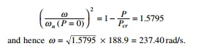
When the axial load = 0 the natural frequency corresponds to
the Euler beam simply supported conditions without axial load and is given by Žēn = 188.9
rad/s. When the axial load is negative, i.e. tension say P = ŌĆ'300 000 N, the
natural frequency is 237.19 which corresponds to the true value
Example 15.4
A cantilever beam shown in Fig.
15.4 is analysed for free vibration. The data E = 200 GPa; mass density
= 7800 kg/m3 L = 4.572 m. The width of the flange =
0.203 m and thickness of flange and web are 0.0178 and 0.0114 m respectively.
Solution
The natural frequency is obtained
as 195.628 rad/s which agrees with 191 rad/s obtained by Wekezer (1987).
Vibration of Timoshenko beam by DQ method
The governing differential equations for free vibration of
Timoshenko beam (including shear deformation and rotary inertia) have been
given in Eq. 13.112 as
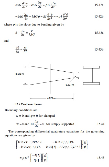
where [I] is the unit matrix and I is the moment
of inertia. Equation 15.45 is written as
╬╗[ B
]{q} = [ D ]{q} --- 15.46
where [B] is of size nn
= 2 ├- n where n is the number of
discrete points. Applying boundary conditions (clamped clamped conditions)
B[nn
+ 1, 1] = 1.0
B[nn
+ 2, n] = 0
B[nn
+ 3, n + 1] = 1.0
B[nn
+ 4, 2n] = 1.0
Using WilsonŌĆÖs method
B[1, nn +
1] = 1.0
B[n,nn +
2] = 1.0
B[n + 1,
nn + 3] = 1.0
B[2n,
nn + 4] = 1.0
Now [B] and [D]
matrices of size nt + 4 because of the application of boundary
conditions. Solving as an eigenvalue problem ╬╗ and hence Žē can be
determined.
Example 15.5
Find the natural frequency of a clamped clamped beam for the
following conditions: L = 10 m, E = 200 GPa, Žü = 7800 kg/m3, assume
unit width (k = 0.83).
Program 15.4: MATLAB program
for free vibration analysis of Timoshenko beam
TIMOSHENKOVIB
% free vibration analysis of
timoshenko beam clc; close all;
ne=20;
no=2;
n=ne+1;
nn=2*n;
nt=nn+4;
m=zeros(n,1);
x=zeros(n,1);
c=zeros(n,n,no);
d=zeros(nt,nt);
e=zeros(nt,nt);
l=10;
e=2e11;
g=.8e11;
ar=2;
ir=0.667;
ak=0.83;
rho=7800;
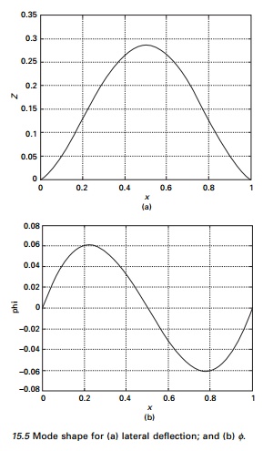
15.5 Mode shape for (a) lateral
deflection; and (b) Žå.
for i=1:n x(i)=0.5*(1-cos((i-1)*pi/ne));
end c=qquadrature(x,n,no);
d(1:n,1:n)=ak*g*ar*c(:,:,2)/l^2;
d(1:n,n+1:nn)=-ak*g*ar*c(:,:,1)/l; d(n+1:nn,1:n)=-ak*g*ar*c(:,:,1)/l;
d(n+1:nn,n+1:nn)=ak*g*ar*eye(n,n)-e*ir*c(:,:,2)/l^2; % %boundary conditions for
fixed end d(nn+1,1)=1.0;
d(nn+2,n)=1.0;
d(nn+3,n+1)=1.0;
d(nn+4,nn)=1.0;
d(1,nn+1)=1.0;
d(n,nn+2)=1.0;
d(n+1,nn+3)=1.0;
d(nn,nn+4)=1.0;
%boundary conditions for ssd end
%d(nn+1,1)=1.0;
%d(nn+2,n)=1.0;
%d(nn+3:nn+3,n+1:nn)=c(1:1,1:n,1)/l;
%d(nn+4:nn+4,n+1:nn)=c(n:n,1:n,1)/l;
%d(1,nn+1)=1.0;
%d(n,nn+2)=1.0;
%for i=1:n
%d(n+i,nn+3)=d(nn+3,n+i);
%d(n+i,nn+4)=d(nn+4,n+i);
%end
e(1:n,1:n)=-rho*ar*eye(n,n);
e(n+1:nn,n+1:nn)=rho*ir*eye(n,n); e(nn+1:nt,1:nt)=0;
ddi=inv(d);
f=ddi*e;
[evv,ev]=eig(f);
disp(ŌĆś natural frequencyŌĆÖ);
wn1=sqrt(1/ev(5,5)) figure(1);
for i=1:n z(i)=evv(i,5);
end plot(x,z) xlabel(ŌĆś x ŌĆś)
ylabel(ŌĆś zŌĆÖ)
title (ŌĆś mode shape of
deflectionŌĆÖ) figure(2);
for i=1:n z(i)=evv(n+i,5);
end plot(x,z) xlabel(ŌĆśxŌĆÖ)
ylabel(ŌĆś phiŌĆÖ)
title(ŌĆś mode shape of phiŌĆÖ)
OUTPUT
natural frequency wn1 =
5.292070310268033e+002
DT method
The concept of the DT method was first introduced some 30
years ago by Pukhov (Chai and Wang 2006) Since then, DT has been used with
success in structural mechanics. The concept of the DT method is readily
available in Russian literature. For a function w(x), DT exists
as
Equation 15.49 is obviously a Taylor series expansion of the
function w(x) about x = 0. The differential technique
essentially converts a differential equation into an algebraic equation,
similar to integral transform methods such as Laplace and Fourier transform.
The final resulting algebraic equations are solved together with boundary
conditions. The transformation can be given by a simple formula as
Transverse vibration of pre-tensioned cable
The governing equation for the transverse vibration of a
pre-tensioned cable
nonlinear equation in terms of ŌĆśaŌĆÖ and linear in terms
of ŌĆścŌĆÖ. Equation 15.59 may be written as A * c = 0, and
since c ŌēĀ 0, A
must be zero where A is the coefficient of c in f (c,
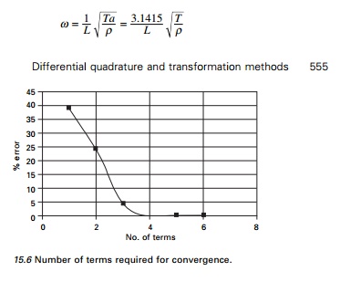
a). It should be noted that a fairly a large number of terms are needed
for convergence of the natural frequency coefficient. Figure 15.6 shows the
convergence of a for different numbers of terms in the summation of Eq.
15.59 and a is obtained as 9.8696. Hence natural frequency is obtained
as
Program 15.5: MATHEMATICA
program for finding the natural frequency of vibration of a pre-tensioned cable
Free vibration analysis of Euler beam
The governing equation is given by Eq. 15.24 as
Boundary conditions
Case 1 Simply supported at both ends
y(0) = 0;
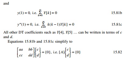
yŌĆ│(0) = 0; y(1) = 0; yŌĆ│ (1) = 0
The DT equivalents are
Y[0] = 0;
Y[1] = c; Y[2] = 0; Y[3] = d
And
since c and d are not zero, for a non-trivial
solution to exist the determinant of the matrix must be zero, i.e.
aa ├- dd ŌĆ' cc ├- bb = 0
--- 15.68
where aa, bb, are
the coefficients of c and d in the equation S = 0 and cc,
dd are the coefficients of c and d in the equation T
= 0. The root of Eq. 15.68 is the solution for the problem.
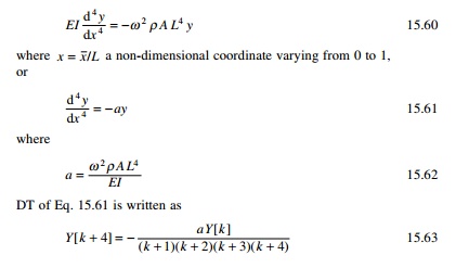
For a beam with simply supported ends a = 97.4091 leads
to natural frequency asyŌĆ▓(1) = 0.
Program
15.6: MATHEMATICA program for finding the natural frequency of vibration of an
Euler beam
Natural
frequency of Euler beam subjected to axial load
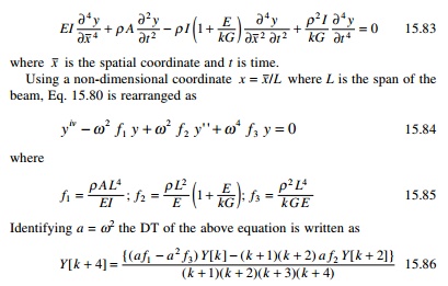
The governing differential equation for an Euler beam
subjected to axial load is given by
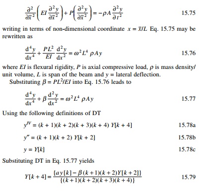
where EI is flexural
rigidity, P is axial compressive load, Žü is mass density/ unit volume, L is span of the beam
and y = lateral deflection.
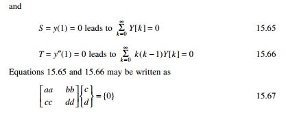
15.19.1Pin roller support
The boundary conditions are
y(0) = yŌĆ│(0) = y(1) = yŌĆ│(1) = 0 --- - - 15.80
This can be interpreted in terms of DT as
Y[0] = 0; Y[2] = 0; Y[1]
= c; Y[3] = d --- ---- 15.81a
where aa, bb are
the coefficients of c and d in Eq. 15.81b and cc and dd
are the coefficients of c and d in Eq. 15.81c. For a numerical
solution to exist, the determinant || A
|| has to be zero and hence a can be
found once ╬▓ is
given. One has to include more terms, say, than 35 in Eq. 15.79 for accuracy.
Example 15.6
Find the buckling load of a
pinnedŌĆ'pinned column given E = 200 GPa; I = 0.000 038 m4;
mass density = 7800 kg/m3, A = 1/7800; span = 12 m. Find the
natural frequency if the axial load is tension of magnitude 300 000 N.
Solution
By trial and error giving various
axial loads the natural frequency is calculated for each axial load and the
load at which natural frequency becomes imaginary is the buckling load. For the
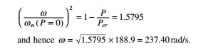
problem, the buckling load is (╬▓ = 9.862) P = 520 895 N, which agrees with (ŽĆ2 EI/L2)
= 520 895 N.
When the axial load = 0 the
natural frequency corresponds to the Euler beam simply supported conditions
without axial load and a is given by a =
97.4091 for which Žēn = 188.9 rad/s.
When the axial load is negative, i.e. tension, say P =
ŌĆ' 300 000 N (╬▓ = ŌĆ'
5.864), the value of a = 153.5 obtained from DT from which natural
frequency is 237.19 which corresponds to the true value
Similarly, other boundary conditions could be tackled.
Program 15.7: MATHEMATICA
program for finding the natural frequency of an Euler beam subjected to axial
load
Natural frequency of a Timoshenko beam
The governing differential equation for free vibration of
Timoshenko beams (including shear deformation and rotary inertia into account)
is given in Eq. 15.42a and 15.42b. Combining these two equations and
identifying y = w = lateral deflection of the beam, the governing
differential equation is given by
For clamped beam the following
boundary conditions are to be applied: y = 0 and Žå = 0 both at x = 0 and x
= 1. In the absence of incorporating the correct boundary conditions, assuming
the shear deformation at the ends of the beam are negligible, we can apply the
boundary conditions as
y = 0 and
yŌĆ▓ = 0, both
at x = 0 and x = 1.
Example 15.7
Find the natural frequency of a clamped-clamped beam for the
following conditions. L = 10 m, E = 200 GPa, Žü = 7800 kg/m3. Assume
unit width (k = 0.83).
Program 15.8: MATHEMATICA
program for finding the natural frequency of a Timoshenko beam
Summary
The DQ and HDQ methods are
applied to solve for natural frequency of strings and, beams with or without
axial load. For finding the natural frequencies, unlike RayleighŌĆ'Ritz methods,
DQ and HDQ methods do not need the construction of an admissible function
that satisfies the boundary conditions a priori. Accurate results are
obtained for the problems even with a small number of discrete points used to
discretize the domain. This approach is convenient for solving problems
governed by higher order differential equations, and matrix operations could be
performed using MATLAB with ease. It is also easy to write algebraic equations
in the place of differential equations and to apply boundary conditions. It is
also explained in this chapter how the Lagrange multiplier method is used to
convert rectangular matrix to square matrix by incorporating boundary
conditions using WilsonŌĆÖs method. Results with high accuracy are obtained in
all study cases and DQM and HDQ methods are computationally efficient. DQM and
HDQ methods are straightforward so the same procedures can be easily employed
for handling problems with the other boundary conditions.
In this chapter, the DT method is also highlighted and its
usefulness demonstrated by solving stability analysis of fully supported
prismatic and non-prismatic piles. It is also shown in this chapter how DT can
be used to convert differential equation to a set of algebraic equations of
recursive nature. It is also shown that, together with boundary conditions,
these equations are solved for natural frequency of various types of problems.
A fairly large number of terms, say 35 to 40, are required for convergence. DT
is efficient and easy to implement, particularly in symbolic program packages
such as MATHEMATICA. Mode shape also could be obtained using Eq. 15.48. It is
expected that DQ, HDQ and DT will be more promising for further development
into efficient and flexible numerical techniques for solving practical
engineering problems in future.
Related Topics