Finite element method

Finite element method in relation to structural dynamics during earthquakes

Abstract: The basic procedure of the finite element method, with application to simple vibration problems, is presented in this chapter. The element stiffness, mass (both consistent and lumped mass) and forced vibration are derived for truss elements, shafts and beam elements. The transformation of the above matrices with respect to the local coordinate system is now transformed to the global system. The equations of motion of the complete system of finite element and the incorporation of boundary conditions are discussed. Relevant computer programs in MATHEMATICA and MATLAB are presented for truss, torsion and beam elements. Although techniques presented are applicable to two- or-three dimensional systems, only the one-dimensional element is treated in this pages.

Key words: discrete element natural frequency, modes, Rayleigh Ritz method, boundary conditions.

Introduction

The finite element method is a powerful numerical method that is used to provide approximations to continuous systems. The disciplines in which the finite element method can be applied include stress analysis, heat transfer, electromagnetic analysis, fluid flow and vibrations. Application of the finite element method to continuous systems requires the systems to be divided into a finite number of discrete elements. Interpolations for the dependent variables are assumed across each element and are chosen to ensure appropriate inter-element continuity. The interpolating functions are developed in terms of unknown values of the dependent variables at discrete points, called nodes which are located for a one-dimensional system at element boundaries. The defined interpolations are used to provide approximation to the dependent variables across the system. Lagrange’s equations are then applied for vibration problems resulting in a set of differential equations for the dependent variables at nodes. Total structure is obtained as assembly of elements.

The term finite element was coined by Prof Clough. Boundary conditions for continuous systems are classified as being of two types:

geometric boundary conditions are those which must be satisfied according to geometric constraints. For example, u(x = 0) = 0 u′(x = 0) = 0 at a fixed end of a cantilever;

•       natural boundary conditions are those that must be satisfied as a result of free and moment balances. For example, EI (∂²u/∂x²) (x = L) = 0 is a moment boundary condition at the free end of a cantilever.

The chosen interpolating function must satisfy geometric boundary conditions.

The type of problem that comes from the realm of structural dynamics is restricted to the calculation of natural frequencies and the corresponding mode shapes of free undamped vibration of common structural components and forms. This requires the development of mass matrix, which will represent the effect of dynamic loading (proportional to the square of frequency) which is set up during vibration. Vibration problems are eigenvalue problems in which eigenvalues represent the square of the natural frequencies and eigenvectors define the shape of the structure when vibrating at a particular frequency.

Dynamic analysis

Basically four different types of problems can be distinguished in the field of dynamics, free vibration, steady state vibration, transient response to known excitations and response to random excitations.

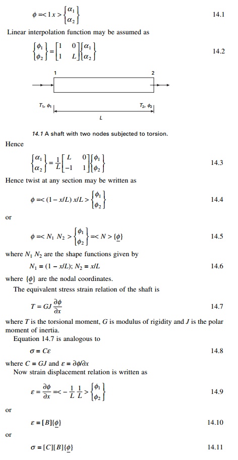
Torsional vibration of a shaft

The shaft element shown in Fig. 14.1 has two nodes at its two ends. The unknown displacements at each end are the angles of twist φ₁, φ₂. The displacement function, which is the angle of twist, is given by

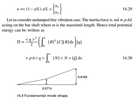
Let us consider undamped free vibration case. The inertia force is Iφ^˙˙ acting on the shaft where I is the mass moment of inertia/unit length. Hence total potential energy can be written as

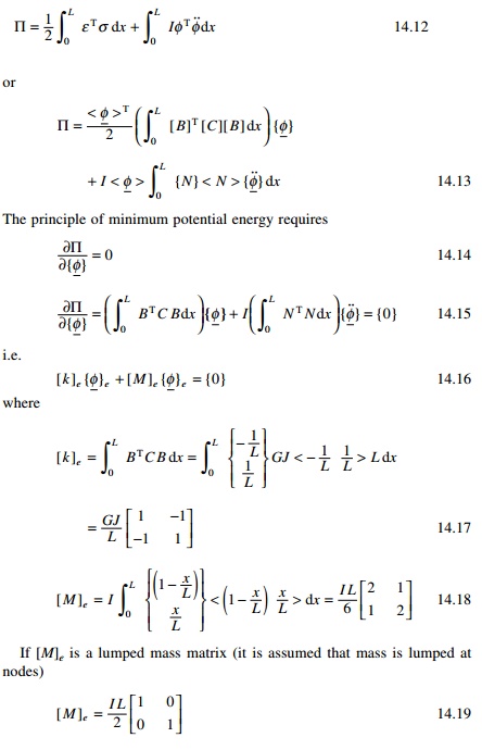
If [M]_e is a lumped mass matrix (it is assumed that mass is lumped at nodes)

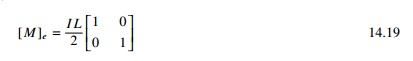
Even though consistent mass is more accurate, lumped mass gives better results because both stiffness and mass are over-estimated, thus resulting in the correct answer.

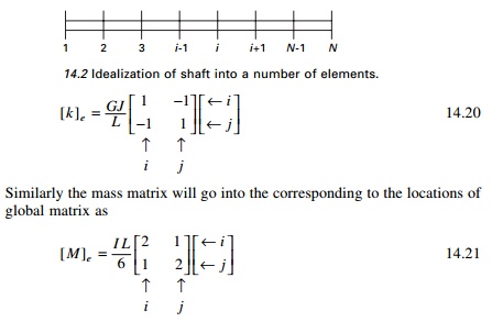
The next step is the assembly of stiffness matrix. Assume that the shaft is idealized into a number of elements as shown in Fig. 14.2 and that each element has two nodes and one degree of freedom at each node. The elements of the stiffness matrix will go into the corresponding position of global stiffness matrix as

When all elements of the element stiffness matrices and mass matrices are assembled, and the boundary conditions incorporated, the final equations of free vibration is as follows

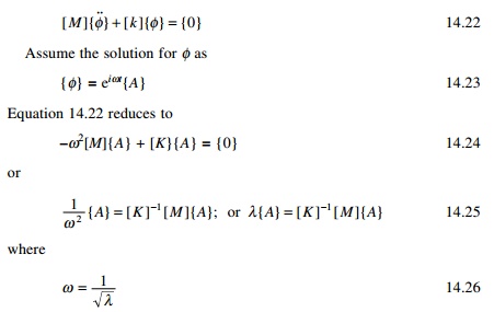
Equation 14.26 is a typical eigenvalue problem.

Example 14.1

A uniform shaft having one end fixed and the other end free is divided into two equal elements as shown in Fig. 14.3. Determine the natural frequency for torsional vibration of the shaft.

Axial vibration of rods

The total degrees of freedom for a bar element are the axial displacements at the ends of the element instead of the angle of twist for torsional vibration. Let u₁, u₂ be the displacements at the left end and right end of an element (see Fig. 14.1). Axial displacement at any section is written as

Hence the stiffness matrix of an element for axial vibration of a rod is the same as torsional vibration of the rod except that GJ is to be replaced by EA.

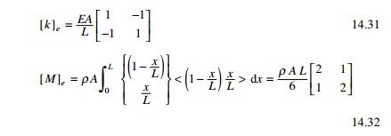
Hence I in the torsional vibration must be replaced by ρA for axial vibration of the rod.

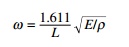
Example 14.2

For the rod shown in Fig 14.3 determine the lowest frequency for longitudinal vibration of the rod by the finite element method by considering two elements. Solution

In the above method, admissible functions are used as basis functions in a Rayleigh�'Ritz approximation to solution of an eigenvalue problem. Sometimes the Rayleigh�'Ritz method is difficult to apply to vibration problems. The assumed modes method, introduced in the next section, is based on application of Lagrange’s equations and leads to the same approximation as that for the same set of interpolating functions as the Rayleigh�'Ritz method. In the next section we will use the finite element method for the longitudinal vibration by the assumed modes method.

14.5      Assumed modes method

Example 14.3

Consider a forced vibration of a longitudinal bar as shown in Fig. 14.5. The displacement u is a function of spatial coordinate x and time t, i.e. u(x, t).

  Program 14.1: MATLAB program for the assumed modes method

%example 14.3

% assumed modes method to determine natural frequencies m mode %shapes, and forced response of tapered bar with attached mass and spring clc;

close all; digits(5); x=sym(‘x’); %parameters

e=200*10^9; % youngs modulus in N/sq.m rho=7800; % mass density in kgm/cu.m l=4.0; % span of the beam in m

m=10; % concentrated mass in kgm k=3*10^7; % spring constant %functions

a=0.001*(1-.005*x);% area in sq.m u(1)=sin(pi*x/(2*l)); % assumed modes u(2)=sin(3*pi*x/(2*l)); u(3)=sin(5*pi*x/(2*l));

%mass and stiffness matrices for i=1:3

for j=1:i c1=subs(u(i),x,l)*subs(u(j),x,l); Mint=rho*a*u(i)*u(j);

Kint=e*a*diff(u(i),x)*diff(u(j),x);

M(i,j)=int(Mint,x,0,l)+m*c1;

K(i,j)=int(Kint,x,0,l)+k*c1;

M(j,i)=M(i,j);

K(j,i)=K(i,j); end

end

disp(‘ stiffness matrix’) K=vpa(K)

disp(‘ mass matrix’) M=vpa(M) K1=double(K); M1=double(M); C=inv(K1)*M1; [V,D]=eig(C);

for i=1:3 w(i)=1/sqrt(D(i,i));

end

disp(‘ natural frequencies in rad/sec’) w=vpa(w);disp(w’)

%Normalize mode shape vectors E=V’*M*V;

for j=1:3 for i=1:3

P(i,j)=V(i,j)/sqrt(E(j,j)); end

end

disp(‘ modal matrix’) P=vpa(P);disp(P) %mode shapes xx=linspace(0,l,37); P1=single(P);

for k=1:37 for i=1:3

v(i,k)=0; for j=1:3

v(i,k)=v(i,k)+P1(j,i)*subs(u(j),x,xx(k)); end

end end

plot(xx,v(1,:),’k’,xx,v(2,:),’*k’,xx,v(3,:),’�'k’); xlabel(‘ x (m)’)

ylabel(‘ w(x) m’)

legend(‘ 1st mode’, ‘2nd mode’, ‘3rd mode’)

Output for example 14.3 stiffness matrix

K =

[ .91319e8, -.29250e8, .30139e8] [ -.29250e8, .57987e9, -.26250e8] [ .30139e8, -.26250e8, .15570e10]

mass matrix M =

[ 25.381, -9.9368, 9.9930] [ -9.9368, 25.437, -9.9368] [ 9.9930, -9.9368, 25.442]

natural frequencies in rad/sec 1895.7 5062.1 8984.0

modal matrix

[ .19713, -.94408e-1, -.53048e-1] [ -.26221e-2, -.20576, .89500e-1] [ .79332e-3, .28353e-1, .22280]

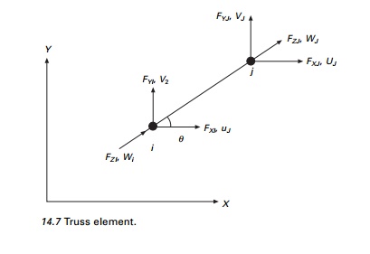
Truss element

Consider a truss element oriented as shown in Fig. 14.7 in the global coordinate system.

14.7.1  Element stiffness and mass matrices

Since the truss element is a bar element subjected to axial forces, the stiffness matrix is given by

The local displacements <w_i w_j> can be written in terms of global displacements as

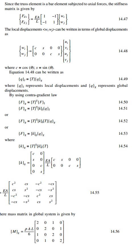
where {q}_l represents local displacements and {q}_g represents global displacements.

By using contra-gradient law

{F}_g = [T]^T{F}_{l                            ---  --}  14.50

{F}_g = [T]^T[k]_l{q}_{l                             ---  --}  14.51

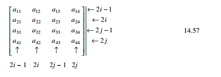
14.7.2  Assembly

The elements of the stiffness matrix and mass matrix will assemble in the proper location of structural stiffness matrix as

3  Application of boundary conditions

•       If any of the degrees of freedom is constrained, the row and column corresponding to that degree of freedom are deleted from the assembled stiffness or mass matrix.

•       Add springs of very high stiffness at the constrained degree of freedom.

•       Use Lagrangian multiplier method to incorporate the constraints.

4  Solve as an eigenvalue problem

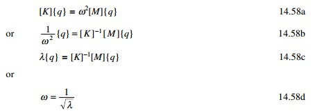
and the corresponding mode shape is also obtained.

Example 14.4

Use the finite element method to obtain the lowest natural frequency for the

truss shown in Fig. 14.8. The data are: L₁ = 1.2 m; L₂ = 2.68 m; L₃ = 2.4 m; L₄ = 1.2 m; θ = 63.43� o ; sin θ = 0.894; cos θ = 0.447 E = 2 �- 10¹¹ N/m²; A = 0.04 m²; ρ = 7600 kg/m³.

Assembling all the elements and eliminating the 1st, 2nd, 7th and 8th (boundary conditions) we get resulting stiffness and mass matrices as

Program 14.2: MATLAB program for free vibration of trusses

 Trussdyn 

 % solution of plane truss free vibration by finite element method

 clc; 

 K=zeros(12,12);

 M=zeros(10,10);

 e=200e9; 

 a=0.04; 

 l1=1.2; 

 rho=7600;

 l2=2.683; 

 l3=2.4; 

 l4=1.2; 

 l5=2.4; 

 % calculate element lengths

 % calculate element stiffness

 k1=PlaneTrussElementStiffness(e,a,l1,0);

 m1=PlaneTrussElementMass(rho,a,l1,0);

 k2=PlaneTrussElementStiffness(e,a,l2,63.43);

 m2=PlaneTrussElementMass(rho,a,l2,63.43);

 k3=PlaneTrussElementStiffness(e,a,l3,90);

 m3=PlaneTrussElementMass(rho,a,l3,90);

 k4=PlaneTrussElementStiffness(e,a,l4,0);

 m4=PlaneTrussElementMass(rho,a,l4,0);

 % assemble element stiffness to global stiffness

 K=PlaneTrussAssemble(K,k1,4,3);

 K=PlaneTrussAssemble(K,k2,1,3);

 K=PlaneTrussAssemble(K,k3,2,3);

K=PlaneTrussAssemble(K,k4,1,2);

M=PlaneTrussAssemble(M,m1,4,3);

M=PlaneTrussAssemble(M,m2,1,3);

M=PlaneTrussAssemble(M,m3,2,3);

M=PlaneTrussAssemble(M,m4,1,2); format long;

ks=1;

% apply boundary conditions for stiffness matrix and mass K(9,1)=ks;

K(10,2)=ks;

K(11,7)=ks;

K(12,8)=ks;

M(9,1)=ks;                    

M(10,2)=ks;

M(11,7)=ks;

M(12,8)=ks;

K(1,9)=ks;

K(2,10)=ks;

K(7,11)=ks;

K(8,12)=ks;

M(1,9)=ks;

M(2,10)=ks;

M(7,11)=ks;

M(8,12)=ks;

invk=inv(K);

km=invk*M;

[ms,ns]=size(M);

% eigen values and eigen vectors [evec,ev]=eig(km);

for i=1:ms ee(i)=1/ev(i,i);

end Qh=max(ee)+0.001; Ql=0;

for i=1:ms for j=1:ms

if ee(j) > Ql & ee(j) < Qh k=j;

Qh=ee(j); else

end end Ql=Qh;

Qh=max(ee)+0.001;

om1(i)=ee(k);

omega(i)=sqrt(ee(k)); for m=1:ms

p1(m,i)=evec(m,k); end

end

%Normalizing the mode shape L=p1'*m*p1;

%develop modal matrix for i=1:ms

for j=1:ms p(i,j)=p1(i,j)/L(j,j);

end end

disp(‘ Natural frequencies in rad/sec’) disp(omega’)

disp(‘ normalized modal vector ‘) disp(p)

function y = PlaneTrussElementStiffness(E,A,L, theta) %PlaneTrussElementStiffness This function returns the element

%stiffness matrix for a plane truss

%element with modulus of elasticity E,

%cross-sectional area A, length L, and

%angle theta (in degrees).

%The size of the element stiffness

%matrix is 4 x 4.

x = theta*pi/180; C = cos(x);

S = sin(x);

y = E*A/L*[C*C C*S -C*C -C*S ; C*S S*S -C*S -S*S ; -C*C -C*S C*C C*S ; -C*S -S*S C*S S*S];

function y = PlaneTrussElementMass(rho,A,L, theta) %PlaneTrussElementStiffness This function returns the mass

%matrix for a plane truss

%element with mass density rho,

%cross-sectional area A, length L, and

%angle theta (in degrees).

%The size of the element stiffness

%matrix is 4 x 4.

x = theta*pi/180; C = cos(x);

S = sin(x);

% for consistent mass use the following

y = (rho*A*L/6)*[2 0 1 0 ; 0 2 0 1 ;1 0 2 0 ; 0 1 0 2]; %for lumped mass use the following %y=(rho*A*L/2)*[1 0 0 0;0 1 0 0;0 0 1 0;0 0 0 1];

function y = PlaneTrussAssemble(K,k,i,j)

%PlaneTrussAssemble This function assembles the element stiffness

%matrix k of the plane truss element with nodes

%i and j into the global stiffness matrix K.

%This function returns the global stiffness

matrix K after the element stiffness matrix

% k is assembled. lm(1)=2*i-1; lm(2)=2*i; lm(3)=2*j-1; lm(4)=2*j;

for m=1:4 ii=lm(m); for n=1:4

jj=lm(n);

K(ii,jj)=K(ii,jj)+k(m,n); end

end

y = K;

OUTPUT

Natural frequencies in rad/sec 1.0e+003 *

0.00100000000000

0.00100000000000

1.25105969735243

3.23474518944287

4.53189428385080

Beam element

Consider a uniform beam element of length L and cross-sectional area A and mass density ρ as shown in Fig. 14.9. The modulus of elasticity of the material is E and I is the second moment of area. The unknown displacement of the element are deflections and rotations at the two ends, in total four degrees of freedom for each element or two degrees of freedom/node. The displacement function is represented by the equation given by

Program 14.3: MATHEMATICA program for evaluation of stiffness matrix, and mass matrix of a beam element

Example 14.5

Find the fundamental frequency of a simply supported uniform beam shown in Fig. 14.10.

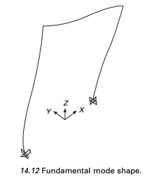
Example 14.6

Set up the system of equation governing free vibration in its own plane of the portal frame shown in Fig. 14.11.

A = 1.851 87 �- 10^�'5; I = 2.857 85 �- 10^�'11; E = 210 GPa;

ρ = 25 613.5 kg/m³; L = 0.2413 m.

Program 14.4: MATLAB program to find the natural frequency of beams or rigid frames

FRAMEDYN

% dynamics of plane frame by finite element method clc;

nj=7;

ne=6;

neq=3*nj;

K=zeros(neq,neq);

M=zeros(neq,neq);

%give nodi and nodj of each member nodi=[1 2 3 4 5 6];

nodj=[2 3 4 5 6 7];

%give the values of e,a,i angle and lengths of members e=210e9;

a=[1.85187e-5 1.85187e-5 1.85187e-5 1.85187e-5 1.85187e-5 1.85187e-5] ; mi=[2.85785e-11 2.85785e-11 2.85785e-11 2.85785e-11 2.85785e-11...

2.85785e-11]; angle=[90 90 0 0 -90 -90];

l=[.12065 .12065 .12065 .12065 .12065 .12065];

%give density of the material

rho=25613.5;

%number of constraint degrees of freedom nbou=6;

%the numbers of constrained degrees of freedom nb=[1 2 3 19 20 21];

%                form 6 x 6 element stiffness and mass matrix and assemble wilson method for n=1:ne

i=nodi(n);

j=nodj(n);

k=PlaneFrameElementStiffness(e,a(n),mi(n),l(n),angle(n));

m=PlaneFrameElementMass(rho,a(n),l(n),angle(n));

K=PlaneFrameAssemble(K,k,i,j);

M=PlaneFrameAssemble(M,m,i,j); end

%apply boundary conditions using wilson method

for i=1:nbou ii=nb(i); for j=1:neq

K(ii,j)=0.0;

K(j,ii)=0.0;

M(ii,j)=0.0;

M(j,ii)=0.0; end K(ii,ii)=1; M(ii,ii)=1;

end

% find inv(K)*M invk=inv(K); km=invk*M;

format long;

%find the eigen values and mode shapes of inv(K)*M [ms,ns]=size(M);

%%eigen values and eigen vectors [evec,ev]=eig(km);

for i=1:ms ee(i)=1/ev(i,i);

end Qh=max(ee)+0.001; Ql=0;

for i=1:ms for j=1:ms

if ee(j) > Ql & ee(j) < Qh k=j;

Qh=ee(j); else

end end Ql=Qh;

Qh=max(ee)+0.001;

om1(i)=ee(k);

omega(i)=sqrt(ee(k)); for m=1:ms

p1(m,i)=evec(m,k); end

end

%Normalizing the mode shape L=p1'*m*p1;

%develop modal matrix for i=1:ms

for j=1:ms p(i,j)=p1(i,j)/L(j,j); end

end

disp(‘ Natural frequencies in rad/sec’) disp(omega’)

disp(‘ normalized modal vector ’) disp(p)

function y = PlaneFrameElementStiffness(E,A,I,L,theta) %PlaneFrameElementStiffness This function returns the element

%stiffness matrix for a plane frame

element with modulus of elasticity E,

%cross-sectional area A, moment of

%inertia I, length L, and angle

%theta (in degrees).

%The size of the element stiffness

%matrix is 6 x 6.

x = theta*pi/180; C = cos(x);

S = sin(x);

w1 = A*C*C + 12*I*S*S/(L*L);

w2 = A*S*S + 12*I*C*C/(L*L);

w3 = (A-12*I/(L*L))*C*S;

w4 = 6*I*S/L;

w5 = 6*I*C/L;

y = E/L*[w1 w3 -w4 -w1 -w3 -w4 ; w3 w2 w5 -w3 -w2 w5 ; -w4 w5 4*I w4 -w5 2*I ; -w1 -w3 w4 w1 w3 w4 ;

-w3 -w2 -w5 w3 w2 -w5 ; -w4 w5 2*I w4 -w5 4*I];

function y = PlaneFrameElementMass(rho,A,l, theta) %PlaneFrameElementMass This function returns the mass

%matrix for a plane frame

%element with mass density rho,

%cross-sectional area A, length L, and

%angle theta (in degrees).

%The size of the element stiffness

%matrix is 6 x 6.

x = theta*pi/180; C = cos(x);

S = sin(x);

% for consistent mass use the following

%mass matrix of frame element consistent matrix

f33 _ 00=[0 . 333,0,0,0 . 167,0,0;0,0 . 37143,0 . 05238*l,0,0 . 12857, - 0.03095*l;0,.05238*l,.00952*l*l,0,0.03095*l,-.00714*l*l;

0.167,0,0,0.333,0,0;0,0.12857,0.03095*l,0,0.37143,-0.05238*l;0,-0.03095*l,-0.00714*l*l,0,-0.05238*l,0.00952*l*l]; t=[C,S,0,0,0,0;-S,C,0,0,0,0;0,0,1,0,0,0;0,0,0,C,S,0;0,0,0,-S,C,0;0,0,0,0,0,1]; n=t’*f33_00*t;

%lumped mass %n=[0.5,0,0,0,0,0;0,.5,0,0,0,0;0,0,0,0,0,0;0,0,0,.5,0,0;0,0,0,0,.5,0;0,0,0,0,0,0]; y=rho*A*l*n;

function y = PlaneFrameAssemble(K,k,i,j)

%PlaneFrameAssemble This function assembles the element stiffness

%matrix k of the plane frame element with nodes

i and j into the global stiffness matrix K.

%This function returns the global stiffness

%matrix K after the element stiffness matrix

%k is assembled.

lm(1)=3*i-2; lm(2)=3*i-1; lm(3)=3*i; lm(4)=3*j-2; lm(5)=3*j-1; lm(6)=3*j; for l=1:6

ii=lm(l); for n=1:6

jj=lm(n);

K(ii,jj)=K(ii,jj)+k(l,n); end

end

y = K;

OUTPUT

Natual frequencies in rad/sec 1.0e+004 *

0.00010000000000

0.01957884271941

0.07771746384284

0.12745125003361

0.13873461021422

0.31352858884033

Forced vibration of a beam

Example 14.7

Use a two element model for the beam to determine the steady state response of the system shown in Fig. 14.13.

clc;

digits(5);

L=8; % length in m

rho=7600; %mass density in kg/cu.m e=2e11; %youngs modulus of the material i=1.6*10^-6; % moment of inertia in m^4 a=3.6*10^-3 % area in m^2

m=20; % mass of hanging block in kg k=3*10^4; % stiffness of discrete spring in N/m s=L/2; %element length

f0=2500; % excitation amplitude in N om=80; %excitation frequency in rad/s disp(‘global mass matrix’)

M=rho*a*s/420*[4*s^2,13*s,-3*s^2,0,0;13*s,312,0,-13*s,0;...

-3*s^2,0,8*s^2,-3*s^2,0;0,-13*s,-3*s^2,4*s^2,0;...

0,0,0,0,420*m/(rho*a*s)]; K=e*i/s^3*[4*s^2,-6*s,2*s^2,0,0;-6*s,24+k*s^3/(e*i),0,6*s,-k*s^3/(e*i);...

2*s^2,0,8*s^2,2*s^2,0;0,6*s,2*s^2,4*s^2,0;...

0,-k*s^3/(e*i),0,0,k*s^3/(e*i)]; M1=vpa(M);disp(M1) K1=vpa(K);disp(K1)

%natural frequencies W2=eig(inv(K)*M); for i=1:5

w(i)=1/sqrt(W2(i)); end

disp(‘ natural frequencies’) w=vpa(w’)

%force vector disp(‘ force vector’)

f=f0*s*[-s/48;13/16;-s/8;-5*s/192;0] %use of undetermined coefficients z=-om^2*M+K;

W=inv(z)*f;

x=linspace(0,L,21); for k=1:21

if x(k) <s xi=x(k)/s;

y(k)=(xi-2*xi^2+xi^3)*W(1)+(3*xi^2-2*xi^3)*W(2); y(k)=y(k)+(-xi^2+xi^3)*W(4);

else xi=(x(k)-s)/s;

y(k)=(1-3*xi^2+2*xi^3)*W(2)+(xi^2-2*xi^2+xi^3)*W(3);

y(k)=y(k)+(-xi^2+xi^3)*W(4); end

end plot(x,y,‘-k’); xlabel(‘ x(m)’);

ylabel(‘w(x) (m)’);

W=vpa(W);

disp(‘ steady state amplitude in m’);disp(W)

OUTPUT

global mass matrix

[ 16.677, 13.550, -12.507, 0., 0.] [ 13.550, 81.298, 0., -13.550, 0.] [ -12.507, 0., 33.353, -12.507, 0.] [ 0., -13.550, -12.507, 16.677, 0.] [ 0., 0., 0., 0., 20.]

[ .32000e6, -.12000e6, .16000e6, 0., 0.]

[ -.12000e6, .15000e6, 0., .12000e6, -30000.] [ .16000e6, 0., .64000e6, .16000e6, 0.]

[ 0., .12000e6, .16000e6, .32000e6, 0.] [ 0., -30000., 0., 0., 30000.]

natural frequencies w =

15.162

42.623

74.044

186.76

339.31

force vector f =

1.0e+003 *

-0.8333 8.1250 -5.0000 -1.0417 0

steady state amplitude in m -.43073e-1

-.10930e-1

.25384e-1 -.22861e-1

.33458e-2

Vibration of a Timoshenko beam

We have already seen that Euler�'Bernoulli’s theory predicts the frequencies for a shallow beam with adequate precision. But with the increasing depth of the beam, the effect of transverse shear deformation and rotary inertia become more important. Many varieties of Timoshenko beam elements have been proposed. It has been observed that the element described below is adequate for practical use.

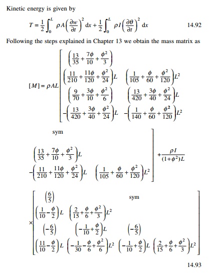
The deflection function is given by

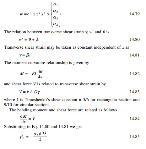
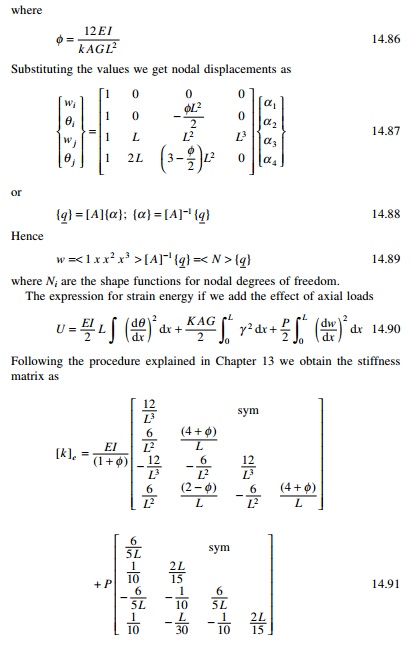
where k is Timoshenko’s shear constant = 5/6 for rectangular section and 9/10 for circular sections.

Example 14.8

Find the fundamental frequency of a Timoshenko beam by using the program ‘Timoshenkovib’ given that

E = 210 GPa; G = 70 GPa; ρ = 7800 kg/m³, A = 1.85187e�'5;

I = 2.85785e�'11; P = 200 N; k = 5/6.

The lowest frequency obtained from the program is 11.7 rad/s.

Program 14.6: MATLAB program to find the frequency of a Timoshenko beam

TIMOSHENKOVIB

% dynamics of Timoshenko beam by finite element method clc;

ne=5;

nj=ne+1;

neq=2*nj;

K=zeros(neq,neq);

M=zeros(neq,neq);

%give nodi and nodj of each member for i=1:nj

nodi(i)=i;

nodj(i)=i+1; end

%give the values of e,g,a,i and lengths of beam e=210e9;

g=70e9;

a=[1.85187e-5 1.85187e-5 1.85187e-5 1.85187e-5 1.85187e-5 1.85187e-5] ; mi=[2.85785e-11 2.85785e-11 2.85785e-11 2.85785e-11 2.85785e-11...

2.85785e-11]; angle=0;

L=10;

for i=1:ne l(i)=L/ne; end

%give density of the material

rho=7800.0;

%give axial load of the member P=200;

%give timoshenko shear constant ko=5/6 for rect ko=9/10 for circular ko=5/6;

%number of constraint degrees of freedom nbou=2;

%the numbers of constrained degrees of freedom nb=[1 2*nj-1];

%                form 6 x 6 element stiffness and mass matrix and assemble wilson method for n=1:ne

i=nodi(n);

j=nodj(n);

phi(n)=12.0*e*mi(n)/(ko*a(n)*g*l(n)^2);

k=TimoshenkoElementStiffness(e,a(n),mi(n),l(n),P,phi(n));

m=TimoshenkoElementMass(rho,a(n),mi(n),l(n),phi(n));

K=TimoshenkoAssemble(K,k,i,j);

M=TimoshenkoAssemble(M,m,i,j); end

%apply boundary conditions using wilson method for i=1:nbou

ii=nb(i); for j=1:neq

K(ii,j)=0.0;

K(j,ii)=0.0;

M(ii,j)=0.0;

M(j,ii)=0.0; end K(ii,ii)=1; M(ii,ii)=1;

end

%find inv(K)*M

invk=inv(K);

km=invk*M; format long;

%find the eigen values and mode shapes of inv(K)*M [ms,ns]=size(M);

%%eigen values and eigen vectors [evec,ev]=eig(km);

for i=1:ms ee(i)=1/ev(i,i);

end Qh=max(ee)+0.001; Ql=0;

for i=1:ms for j=1:ms

if ee(j) > Ql & ee(j) < Qh kl=j;

Qh=ee(j); else

end end Ql=Qh;

Qh=max(ee)+0.001;

om1(i)=ee(kl);

omega(i)=sqrt(ee(kl)); for lm=1:ms

p1(lm,i)=evec(lm,kl);

end

end

%Normalizing the mode shape

LL=p1'*M*p1;

%develop modal matrix

for i=1:ms

for j=1:ms

p(i,j)=p1(i,j)/LL(j,j);

end

end

disp(‘ Natural frequencies in rad/sec’)

disp(omega’)

disp(‘ normalized modal vector ‘)

disp(p)

function y = TimoshenkoElementStiffness(E,A,I,L,P,phi)

%TimoshenkoElementStiffness This function returns the element

% stiffness matrix for a Timoshenko beam element

% element with modulus of elasticity E,

% cross-sectional area A, moment of

% inertia I, length L, and angle

% theta (in degrees).

% The size of the element stiffness

% matrix is 6 x 6.

con=E*I/(1+phi);

w1 = 12*con/L^3+1.2*P/L;

w2 = 6*con/L^2+P/10;

w3 = con*(4+phi)/L+2*P*L/15;

w4 = con*(2-phi)/L-P*L/30;

y = [w1,w2,-w1,w2;w2,w3,-w2,w4;-w1,-w2,w1,-w2;w2,w4,-w2,w3];

function y = TimoshenkoElementMass(rho,A,I,l,phi) %TimoshenkoElement Mass matrix This function returns the mass

%matrix for a Timoshenko beam

%element with mass density rho,

%cross-sectional area A, length L, and

%angle theta (in degrees).

%The size of the element stiffness

matrix is 4 x 4. a(1,1)=13/35+7*phi/10+phi^2/3; a(1,2)=(11/210+11*phi/120+phi^2/24)*l; a(1,3)=9/70+3*phi/10+phi^2/6; a(1,4)=-(13/420+3*phi/40+phi^2/24)*l;

a(2,2)=(1/105+phi/60+phi^2/120)*l^2;

a(2,3)=(13/420+3*phi/40+phi^2/24)*l; a(2,4)=-(1/140+phi/60+phi^2/120)*l^2; a(3,3)=(13/35+7*phi/10+phi^2/3); a(3,4)=-(11/210+11*phi/120+phi^2/24); a(4,4)=(1/105+phi/60+phi^2/120)*l^2; b(1,1)=1.2;

b(1,2)=(0.1-0.5*phi)*l; b(1,3)=-1.2; b(1,4)=(0.1-0.5*phi)*l; b(2,2)=(2/15+phi/6+phi^2/3)*l^2; b(2,3)=(-1/10+phi/2)*l; b(2,4)=(-1/30-phi/6+phi^2/6)*l^2; b(3,3)=1.2; b(3,4)=(-0.1+0.5*phi)*l; b(4,4)=(2/15+phi/6+phi^2/3)*l^2; for i=2:4

for j=1:(i-1) a(i,j)=a(j,i); b(i,j)=b(j,i);

end end

y=(rho*A*l)*a+(rho*I/((1+phi^2)*l))*b;

function y = TimoshenkoAssemble(K,k,i,j)

%Timoshenko beam This function assembles the element stiffness

%matrix k of the Timoshenko beam with nodes

%i and j into the global stiffness matrix K.

%This function returns the global stiffness

%matrix K after the element stiffness matrix

%k is assembled.

lm(1)=2*i-1; lm(2)=2*i; lm(3)=2*j-1; lm(4)=2*j; for l=1:4

ii=lm(l); for n=1:4

jj=lm(n);

K(ii,jj)=K(ii,jj)+k(l,n); end

end

y = K;

end

y = K;

OUTPUT

Natual frequencies in rad/sec 1.0e+002 * 0.01000000000000 0.11701648818926 0.23474939088448 0.35376511095837 0.47263579452189 0.61764685636320 0.77724091967848 0.93007476129177 1.12011725011258 1.36597976298605 1.66895296196556 1.66895296196556

Summary

In this chapter, free and forced vibrations of beams, trusses and frames are discussed. In the next chapter, we will apply other numerical methods such as differential quadrature and transformation methods to find the natural frequencies of structures.