Time history response by mode superposition

Time history response by mode superposition in relation to structural dynamics during earthquakes

Abstract: In this page, the mode superposition method using the mode displacement and the mode acceleration methods is used to find the response of the structure with classical damping. In addition, numerical methods discussed in previous pages for a single-degree-of-freedom system are extended to find the dynamic response for a multiple-degrees-of-freedom system. Relevant programs in MATLAB are also given.

Key words: normal coordinate, classical damping, time history, response spectrum, SRSS rule, CQC rule.

Introduction

In the multi-storey building or in any system having n degrees of freedom, if principalmodes (normal modes) are used as generalized coordinates, the n dynamic equilibrium equations will be uncoupled. Hence each uncoupled equation can be solved independently as each equation contains one degree of freedom only. One can apply any one of the numerical methods to determine the response of a single-degree-of-freedom system. The response of a multiple-degrees-of-freedom (MDOF) system is obtained by mode superposition by summing the response of the individual modes. This procedure of dynamic analysis is referred to as the mode superposition method, normal mode method or simply modal analysis.

Limitations

Modal analysis is valid for linear systems only. Damping in the system must be proportional to mass and stiffness and this damping is known as classical damping. There are two forms of mode superposition method:

•       mode displacement method;

•       mode acceleration method.

The mode displacement method is based on stiffness formulation and the mode acceleration method is based on the flexibility approach. Hence the second method is not widely used. We will discuss mode displacement method first followed by the mode acceleration method.

It is observed in structural or mechanical systems that in most types of dynamic loadings, the contributions of the various modes to the dynamic response are the greatest for lowest frequencies and tend to decrease for higher frequencies. Hence for practical applications, it is usually not necessary to include any of the higher modes of vibration in the superposition process.

Mode displacement method for uncoupled system

Method 1

The dynamic equation of motion for an n degree of freedom system may be written as

[m]{u} + [k ]{u} = {F(t )} = {F} f (t )                   ---- 12.1

where k and m are the symmetric stiffness and mass matrices respectively, u , u˙˙ are displacement and acceleration in physical coordinates respectively, F(t) is the external force vector. Equation 12.1 is a coupled equation since it cannot be solved independently, only simultaneously. The coupling may be due to stiffness coupling or inertial coupling. The mass matrix will be uncoupled for a lumped mass system and coupled for a consistent mass system. The mode superposition method cannot be applied to the coupled form of equation such as Eq. 12.1.

It is therefore necessary to find a coordinate system which will exhibit neither stiffness coupling nor mass coupling which is the main essence of mode superposition method. The coordinates that enable the decoupling of the equations of motion are called ‘principal coordinates’ or ‘normal coordinates’.

To uncouple the equations we introduce an alternative set of coordinates y such that

y = y(u1, u2,…, un)                        --- 12.2

i.e. the actual generalized coordinate u can be written in terms of new coordinates y as

{u} = [ψ]{y}              - - - -       12.3

where [ψ] is the modal matrix determined from the solution of eigenvalue problem. Each column vector of denotes the normalized eigenvector corresponding to that particular mode. Hence u can be written as

{u} = [ψ]{y}                           --- 12.4

Hence transforming the equations of motion Eq. 12.1 from physical coordinates to normal coordinates as

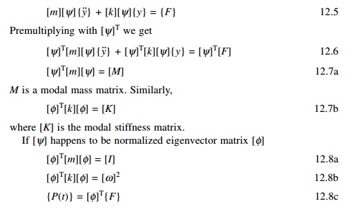
P(t) is called modal force vector or modal participation factor.

Since the modal mass = I and modal stiffness matrices = [ Ï‰ n2 ] are diagonal can be written in a uncoupled equations as

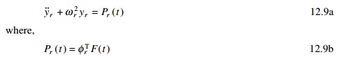
The complete response for the rth mode can be expressed as the sum of response due to initial conditions and the modal response due to Pr(t).

The solution of Eq. 12.9a is written as

yr = ycr + ypr                --- 12.10

where

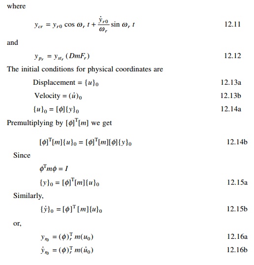
Thus complete response for the rth mode in normal coordinate can be represented by the Duhamel integral expression as

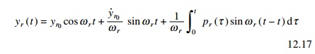
The procedure discussed in previous pages for evaluating an integral is also applicable to Eq. 12.17. However for random dynamic excitation, it is generally necessary to employ one of the numerical techniques discussed in earlier chapters to obtain the time history response.

Now the exact response in physical coordinate is obtained by summing up all the individual modal responses in normal coordinates given by

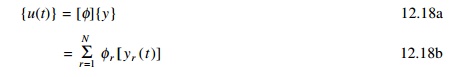
Modal analysis is effective when only a few modes of the system are required to render an accurate solution. In the case of tall buildings having hundreds of degrees of freedom, the entire building possesses 100 eigen pairs (i.e. 100 eigenvalues and 100 eigenvectors) that describe the normal vibration mode. If it is known that frequency content of excitation force is in the vicinity of the lowest few frequencies of the building, the higher modes will not be excited and the force response can be determined by superposition of only these few low frequency modes. Hence the displacement u(t) is given as

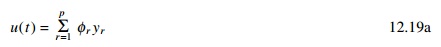
where p â‰¤ N. Suppose the excited force vector is given as

Modal participation factor

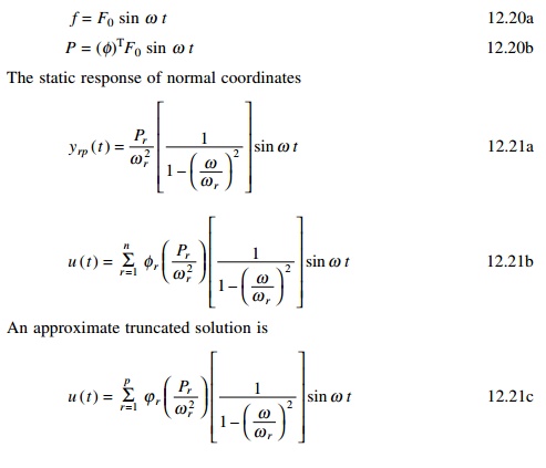
The forced response of an MDOF system is expressed in Eq. 12.21b as

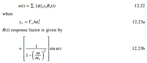
Î'r is called modal participation factor and is particular useful when used in conjunction with the response spectrum analysis of MDOF systems.

Method 2 due to Chopra

Dynamic equation of motion of an n-degrees-of-freedom system is given by

[ m ]{u} + [ k ]{u} = { F} f ( t )                    ---   12.24

Assume the force vector is written in terms of normalized eigenvector as

{F} = âˆ' Î'ι[m]{φ}I                 --- 12.25

Premultiplying both sides with {φ}nT we get

Î'n  = {φ} nT { F}             --- 12.26

where Î'n is known as the modal participation factor corresponding to mode n. Similarly all the modal participation factors can be found.

Now the force contribution for each mode can be found out as

[F] = [m][φ][Î']        -- - 12.27

where [Î'] is a diagonal matrix consisting of all modal participation factors. [F] contains n â€' columns = number of degrees of freedom of the system. The first column of [F] may be viewed as an expression of the distribution of {F} of applied force in terms of force distribution {F1} associated with natural period Ï‰n1. The force vector {Fnf (t)} produces a response only in the nth mode and no response in other modes. The dynamic response in thenth mode is entirely due to partial force vector {Fnf (t)}

  Mode superposition solution for systems with classical damping

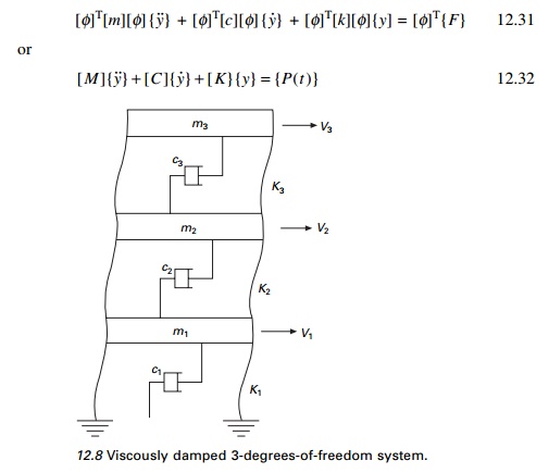
Consider a multi-storey frame shown in Fig. 12.8. Usually damping which is inherent property of the structure is present. In addition to stiffness, and masses the damping of each floor is given by c1, c2, c3 respectively.

The equation of motion for a general as shown in viscously damped MDOF Fig. 12.8 is expressed as

[m ]{u˙˙} + [c ]{uË™} + [k ]{u} = { f (t )}     --- 12.28

where M is = mass matrix

c is = damping matrix k is = stiffness matrix

Writing generalized coordinates in terms of ‘normal’ coordinates as

{u} = [φ]{y}          --- 12.29

Substituting in terms of normalized coordinates Eq. 12.28 becomes

[m ][φ ]{y} + [c ][φ ]{y} + [k ][φ ]{y} = {F (t )}               ---- 12.30

Premultiplying with [φ] we get

where M, C and K are the generalized mass, generalized damping and generalized stiffness matrices. If [φ] is the normalized eigenvector

[φ]T[m][φ] = [I]

[φ]T[K][φ] = [ω2]                 ---- 12.33

C is an n Ã- n symmetric matrix that is diagonal only for a special case of [c]. This special case of [c] is referred to a classical damping or proportional damping for which [c] is proportional to m and k as

where [C] is a diagonal matrix and is called the modal damping matrix, in which,

cr  = Î± + Î² ω r2                 ---- 12.35

Cr is called the modal damping coefficient for rth mode. Assume modal damping factor is given by

The solution of Eq. 12.38 for the rth mode can be expressed by the same form as a single-degree-of-freedom (SDOF) system and the solution is given by

Frequently, in the absence of more definite information about damping, a reasonable value for modal damping as Eq. 12.38 is simply assumed to be valid.

If the solution of ‘n’ modal equations given by Eq. 12.38 are substituted in Eq. 12.29

Then the exact system response u(t) in physical coordinates for all n mode is obtained. However, if only p modes are retained in the solution then

rather than Eq. 12.41 is used to define the truncated response. The resulting mode superposition solution omits the contribution of the modes (p + 1) to n.

The damping discussed above is called Rayleigh damping, which is just one example of proportional damping. This damping is also referred to as classical damping, orthogonal damping and modal damping.

In Rayleigh damping the modal damping matrix [c] is defined as

Rayleigh damping is therefore defined for an MDOF system by specifying for two different unequal frequencies of vibration and solving by simultaneous solution of the equation

Solving Eqs 12.45a and 12.45b we get Î± and Î² and hence [c] matrix is defined. It is also seen in Eq. 12.44 that contribution of mass in damping is

inversely proportional to Ï‰r and contribution of stiffness is proportional to

ωr.

Therefore for large Ï‰r the stiffness proportional term determines the system damping. This trend generally leads to unrealistically high damping ratios in higher modes. For a large MDOF system fortunately the modal superposition methods, we consider p < < n modes only and hence damping in the higher modes is generally not a critical issue. In modal analysis it is not necessary to formulate or explicitly give the equation for [C] displacement since the values of Î¶r are required. But [C] is required for dynamic response of MDOF system by direct numerical integration procedure.

Numerical evaluation of modal response

The numerical integration procedures discussed in earlier chapters for an SDOF system can readily be applied to MDOF systems. Using modal analysis we get n independent (uncoupled) differential equations which are then evaluated at discrete time intervals by any numerical procedure. These normal coordinates are transformed back to physical coordinatesu and updated after each time step.

One has to resort to numerical integration procedure since the forcing function is arbitrary and cannot be expressed by means of a simple analytical expression. The algorithm is given in Table 12.1. As has been already seen for accuracy t â‰¤ Tn/10 should be selected where Tn is the natural period corresponding to highest ratio mode associated with the system. When fewer modes are considered âˆ†t â‰¤ Tp/10 where Tp is the period of pth mode.

Program 12.1: MATLAB program for dynamic response using modal superposition

% program to get dynamic response of MDOF using modal superposition %force.dat contains data time, force1, force2, force3

clc; close all;

m=[18348 0 0;0 13761 0;0 0 9174]; [nd,nd]=size(m);

disp(‘ mass matrix’) m

%if forces are acting at degrees of freedom force=‘force.dat’

f=load(force);

%if base ground acceleration is given

%dis=‘disp.dat’

%di=load(dis);

%% convert to equivalent nodal loads

%for i=1:nd

%f(:,i)=-di*m(i,i);

%end

%you can give stiffness matrix disp(‘ stiffness matrix’)

k=[.74504e8 -.64228e8 0;-.64228e8 .14746e9 -.8324e8;0 -.8324e8 .8324e8]; k

a=inv(k);

%or you can given flexibility matrix directly

%a=[.75 .5 .25;.5 1 .5;.25 .5 .75];

disp(‘ flexibility matrix’) a

cc=a*m;

[ms,ns]=size(m);

%eigen values and eigen vectors [V,D]=eig(cc);

for i=1:ms e(i)=1/D(i,i);

end Qh=max(e)+0.001; Ql=0;

for i=1:ms for j=1:ms

if e(j) > Ql & e(j) < Qh kk=j;

Qh=e(j); else

end end Ql=Qh;

Qh=max(e)+0.001;

om1(i)=e(kk);

omega(i)=sqrt(e(kk)); for l=1:ms

p1(l,i)=V(l,kk); end

end

%Normalizing the mode shape L=p1'*m*p1;

%develop modal matrix for i=1:ms

for j=1:ms ph(i,j)=p1(i,j)/sqrt(L(j,j));

end end

disp(‘ Natural frequencies in rad/sec’) disp(omega)

disp(‘ normalized modal vector’) disp(ph)

ph’*m*ph

%give alpha and beta alpha=0.6978; beta=9.4e-4;

disp(‘ damping matrix’) cd=alpha*m+beta*k; cd

for i=1:ms zeta(i)=0.5*(alpha/omega(i)+beta*omega(i));

end

%give initial displacements and velocities of all degrees of freedom xin=[0; 0.0; 0.0];

vin=[.0; 0.0; 0];

disp(‘ initial displacements of all degrees of freedom’) xin

disp(‘ initial velocities of all degrees of freedom’) vin

xmin=ph’*m*xin; vmin=ph’*m*vin;

%define forces at various times at all degrees of freedom dt=0.02;

ttot=5.0;

p=f*ph; for ii=1:nd

x(1,ii)=xmin(ii,1);

x1(1,ii)=vmin(ii,1);

c=2.0*zeta(ii)*omega(ii); x2(1,ii)=p(1,ii)-c*x1(1,ii)-omega(ii)^2*x(1,ii);

ks=omega(ii)^2+2.0*c/dt+4.0/(dt^2);

ic=1;

for t=0:dt:ttot-dt dps=p(ic+1,ii)+(4.0*x(ic,ii)/dt^2+4.0*x1(ic,ii)/dt...

+x2(ic,ii)+c*2.0*x(ic,ii)/dt+x1(ic,ii));

x(ic+1,ii)=dps/ks; x2(ic+1,ii)=(4.0/dt^2)*(x(ic+1,ii)-x(ic,ii)-...

dt*x1(ic,ii))-x2(ic,ii); x1(ic+1,ii)=(2.0/dt)*(x(ic+1,ii)-x(ic,ii))-x1(ic,ii); ic=ic+1;

end end u=x*ph’; v=x1*ph’;

acn=x2*ph’; tt=linspace(0,5,251); figure(1); plot(tt,u(:,3),‘k’) xlabel(‘ time in secs’);

ylabel(‘ roof displacement in m’);

title(‘ displacement response of the roof’) figure(2);

plot(tt,v(:,3),‘k’) xlabel(‘ time in secs’);

ylabel(‘ roof velocity in m/sec’); title(‘ velocity response of the roof’) figure(3);

plot(tt,acn(:,3),‘k’) xlabel(‘ time in secs’);

ylabel(‘ roof acceleration in m/sq.sec’); title(‘ acceleration response of the roof’)

OUTPUT OF MATLAB

mass matrix

m =

18348         0     0

0                   13761  0

0                   0 9174

force = force.dat

stiffness matrix

k =             

74504000   â€'64228000 0       

â€'64228000 147460000 â€'83240000

0        â€'83240000 83240000

flexibility matrix 

a =             

1.0e-006 *           

0.0974        0.0974        0.0974

0.0974        0.1130        0.1130

0.0974        0.1130        0.1250

damping matrix            

cd =           

1.0e+005 *          

0.8284        â€'0.6037      0

â€'0.6037      1.4821        â€'0.7825

0        â€'0.7825      0.8465

Natural frequencies in rad/sec

15.3317      74.7946      134.2407

normalized modal vector        

â€'0.0046      â€'0.0055      0.0016

â€'0.0051      0.0024        â€'0.0064

â€'0.0052      0.0063        0.0065

ans =          

1.0000        0.0000        â€'0.0000

0.0000        1.0000        0.0000

â€'0.0000      0.0000        1.0000

initial displacements of all degrees of freedom

xin =

0

0

0

initial velocities of all degrees of freedom

vin =

0

0

0

Dynamic analysis using direct integration methods

In Chapter 7, we saw the dynamic analysis of a SDOF system using the direct integration method. Here Newmark’s constant and linear acceleration methods can be extended to get dynamic response for MDOF systems. Table 12.2 gives the algorithm for the dynamic analysis of MDOF systems using Newmark’s method. This algorithm can be modified so as to apply Wilson-θ or any other numerical method discussed in previous pges.

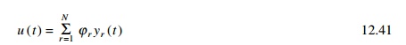
The program developed in MATLAB is applied to Example 12.4 and the dynamic displacement, velocity and acceleration response of the roof are obtained as shown in Fig. 12.12.

Program 12.2: MATLAB program for finding dynamic response of MDOF using direct integration method (Newmark’s method)

%dynamic analysis using direct integration method

%input mass matrix

*force.dat contains data for forces as time, force1, force2,force3 clc;

close all

m=[18438.6 0 0;0 13761 0;0 0 9174]; disp(‘ mass matrix’)

m [ns,ms]=size(m);

%if forces are acting at degrees of freedom force=‘force.dat’

f=load(force);

%disp(‘ force at various degrees of freedom’);

%f;

%if base ground acceleration is given

%dis=‘disp.dat’

%di=load(dis)

%% convert to equivalent nodal loads

%for i=1:ns

%f(:,i)=-di*m(i,i)

%end

%input damping matrix

c=100000*[0.82836 -0.6037 0;-0.6037 1.4821 -0.7824;0 -0.7824 0.84647]; disp(‘ damping matrix’)

%input stiffness matrix

k=[74504937 -64228394 0;-64228394 147468394 -83240000;0 -83240000 83240000];

disp(‘ stiffness matrix’) k

format long; kim=inv(k)*m; [evec,ev]=eig(kim);

for i=1:ns omega(i)=1/sqrt(ev(i,i));

end

disp(‘ natural frequencies’) omega

% give gamma=0.5 and beta=0.25 for Newmark average accln method %gama=0.5;

%beta=0.25;

%give gamma=0.5 and beta=0.1667 for Newmark linear accln method gama=0.5;

beta=0.167;

%give initial conditions for displacements u0=[0.0 0.0 0.0];

disp(‘ initial displacements’) u0

%give initial condition for velocities v0=[0. 0. 0.];

disp(‘ initial velocities’) v0

for i=1:ns a0=inv(m)*(f(1,:)’-c*v0'-k*u0');

end dt=0.02;

kba=k+(gama/(beta*dt))*c+(1/(beta*dt*dt))*m;

kin=inv(kba);

aa=(1/(beta*dt))*m+(gama/beta)*c; bb=(1/(2.0*beta))*m+dt*(gama/(2.0*beta)-1)*c; u(1,:)=u0;

v(1,:)=v0;

a(1,:)=a0; for i=2:251

df(i,:)=f(i,:)-f(i-1,:)+v(i-1,:)*aa’+a(i-1,:)*bb’; du(i,:)=df(i,:)*kin;

dv(i,:)=(gama/(beta*dt))*du(i,:)-(gama/beta)*v(i-1,:)+dt*(1-gama/ (2.0*beta))*a(i-1,:);

da(i,:)=(1/(beta*dt^2))*du(i,:)-(1/(beta*dt))*v(i-1,:)-(1/(2.0*beta))*a(i-1,:); u(i,:)=u(i-1,:)+du(i,:);

v(i,:)=v(i-1,:)+dv(i,:); a(i,:)=a(i-1,:)+da(i,:);

end tt=linspace(0,5,251); figure(1); plot(tt,u(:,3),’k’); xlabel(‘ time in secs’);

ylabel(‘ roof displacement’);

title(‘ displacement response of the roof’); figure(2);

plot(tt,v(:,3),’k’); xlabel(‘ time in secs’); ylabel(‘ roof velocity’);

title(‘velocity response of the roof’); figure(3);

plot(tt,a(:,3),’k’); xlabel(‘ time in secs’);

ylabel(‘ roof acceleration’);

title(‘ acceleration response of the roof’)

force =

force.dat

damping matrix

c =             

82836       â€'60370         0

â€'60370     148210         â€'78240

0               â€'78240         84647

stiffness matrix

k =             

74504937 â€'64228394 0         

â€'64228394 147468394 â€'83240000

0               â€'83240000   83240000

natural frequencies

omega =

1.0e+002 *

0.15323852988388       0.7469278455770         1.34226456460257

initial displacements

u0 =

0               0         0

initial velocities

v0 =

0               0         0

Normal mode response to support motions

In many structures there is a great interest in studying the response of MDOF systems due to support motions such as the earthquake response of structures (see Fig. 12.13).

Let ug be the ground displacement due to earthquake motion. The system equilibrium equations is physical components is written as

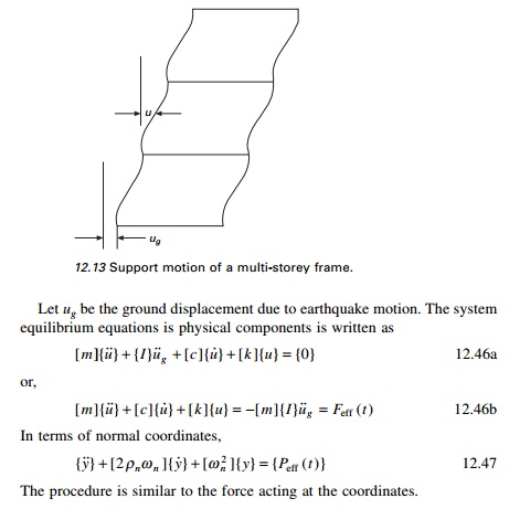
The procedure is similar to the force acting at the coordinates.

Example 12.5

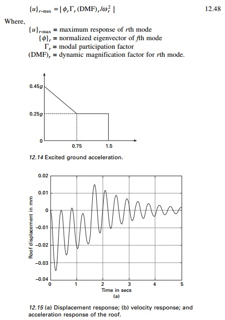
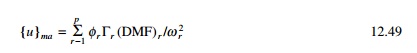
The base of the three storeyed shear frame building shown in Fig.12.9 is excited by horizontal ground acceleration u˙˙g shown in Fig. 12.14. Determine the dynamic response of the structure by mode superposition method. Plot the histories for relative displacement, relative velocity and total absolute acceleration for the top level of the building for the time interval 0 â‰¤ t â‰¤ 5.

Solution

The displacement, velocity and total acceleration history at the roof are shown in Fig. 12.15.

Response spectrum analysis

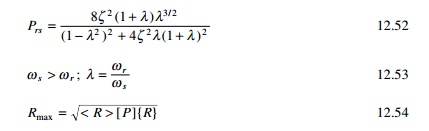
In Previous pages we discussed the response spectra or shock spectra for a specific dynamic disturbance particular for an SDOF system. The technique is also applicable to MDOF systems. Usually the design engineer is interested in finding the maximum response of a system to a specified input. In such cases response spectrum analysis is useful. The maximum modal response of rth mode of an MDOF system to a specified input is expressed in physical coordinates as

An upper bound for the total response may be obtained by summing numerically the maximum response for each mode. Hence maximum response can be expressed as

The numerical sum as given in Eq. 12.49 is a very conservative estimate. This shows that maximum response for all modes occur simultaneously.

This is neither reasonable nor correct. Many statistical methods for combining the maximum modal response have been developed and several of these modal combinations will be discussed later. A popular method is square root of sum of squares (SRSS) given by

The SRSS method for combining modal maximum has been shown to render acceleration approximation to two-dimensional structural systems exhibiting well-separated vibration frequencies. For three-dimensional systems and other systems with closely spaced modes, the complete quadratic combination (CQC) method renders significant improvement in estimating the response. (Two consecutive modes are assumed as closely spaced of their corresponding frequencies differ from each other by 10% or less of the lower frequency.) The CQC combination is expressed as

where Rr and Rs are the peak values or the particular response for the rth and sth modes respectively. For constant damping Î¶ = Î¶1 = Î¶2 = â€¦ = Î¶p and Prs is given is

Mode acceleration method

An alternative form of mode superposition method is mode acceleration method. Since it is a flexibility approach, it is not usually employed in dynamics. Compared with mode superposition analysis it exhibits improved convergence characteristics. In this method we require fewer vibration modes.

The equation of motion can be written as

where [K]â€'1 = [a]. If the acceleration vector is approximately uˆ then truncated mode acceleration solution is given by

But u˙˙(t ) (physical coordinates) can be written in terms of normalized coordinates as

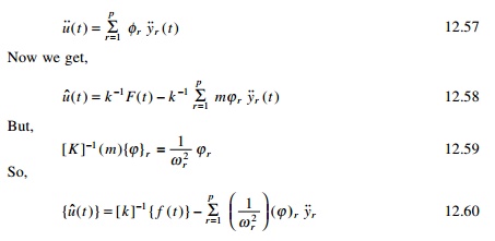
The first term of Eq. 12.60 represents the pseudo-static response and the second term is the mode acceleration, which gives the method its name. Since Ï‰ is in the denominator, this method provides quadratic convergence. Even though it is enough to consider ‘p’ modes, it is also important to consider all the roots whose frequencies are close proximity to any excitation frequency.

Summary

In this page, time history analysis has been carried out by modal superposition and numerical integration methods. In addition, the modal acceleration method is also applied to find the dynamic response of the structures.