Response of structures to impulsive loads

Response of structures to impulsive loads

Abstract: Impulsive force is a force of large magnitude that acts over a short time interval. In practice, vehicles and cranes are subjected to impulsive loads. In this chapter, the response of the single-degree-of-freedom system with or without damping subjected to impulsive loads is considered. The concept of response spectrum, which is a very useful tool in the design, is also illustrated.

Key words: impulsive loads, dynamic magnification factor, shear frame, Duhamel integral, ramp, response spectrum, Laplace transform.

Introduction

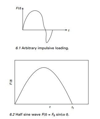
An impulsive load consists of a single principal impulse as illustrated in Fig. 6.1. Such a load is generally of short duration. Vehicles and cranes, etc., are subjected to impulsive loads. The maximum response is reached due to impulsive loads within a short period of time before damping forces absorb much energy. Hence for this reason only, an undamped response to impulsive loads will be considered, and for completeness an under-damped system subjected to impulsive load will also be discussed.

Impulsive loading �' sine wave

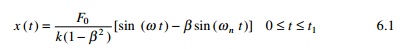
Consider a sine wave impulse as shown in Fig. 6.2 with the duration of sine pulse as t₁.

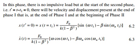
1.Phase I

During this phase, the structure is subjected to harmonic loading starting from rest. The undamped response including transient and steady state may be obtained as

where β is the frequency ratio, ω_n is the natural frequency of the system and t₁ is the time duration of the pulse.

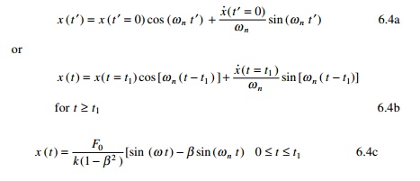
2.Phase II

In this phase, there is no impulsive load but at the start of the second phase, i.e. t′ = t�'t₁ = 0, there will be velocity and displacement present at the end of phase I that is, at the end of Phase I and at the beginning of Phase II

We have seen in 4th previous pages the response of undamped system due to initial velocity and initial displacement is given by

To find the maximum response velocity must be equated to zero. Usually this occurs in Phase I.

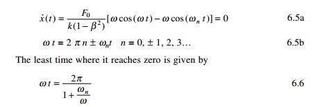
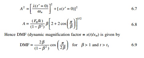
Hence maximum displacement can be obtained by substituting ω t in Eq. 6.6 in Eq. 6.4c. The result is valid only if ω t < 1 or β < 1, i.e. ω_n < ω. For β > 1 the maximum response occurs in Phase II. The amplitude of vibration is given by

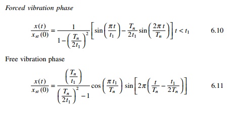
3. Case 1 When t₁/T_n ≠ ½

Forced vibration phase

Free vibration phase

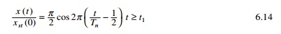
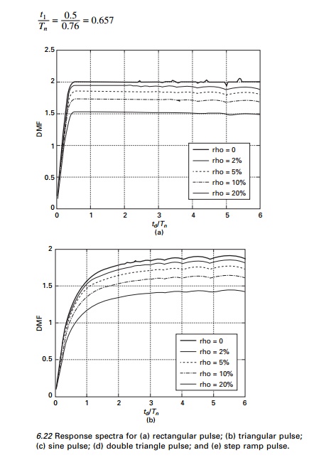
4.Case 2 When t₁/T_n = 1/2

Forced vibration phase

Free vibration phase

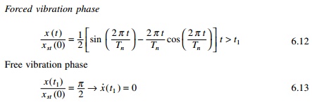
The above equation implies that the displacement in the forced vibration phase reaches a maximum at the end of the phase.

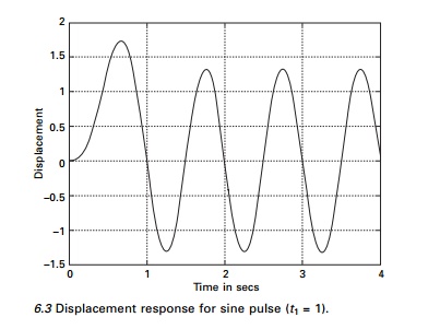
The displacement response for sine pulse with duration of pulse t₁ = 1s is shown in Fig. 6.3.

Maximum response

The maximum values of response over each of the two phases, forced vibration and free vibration, are determined separately. The larger of the two values is the overall maximum response.

A program in MATLAB to obtain the maximum response for various values of t₁/T_n is given below.

Program 6.1: MATLAB program to obtain maximum response for half sine cycle pulse

%Program to obtain maximum response for half cycle pulse force %For various values of t1/Tn- Tn assumed as 1 rad/sec

for j=1:97 c(j)=(j-1)*0.0625 d=1/c(j); t1=c(j);

% time increment dt=0.002;

if c(j)==0.50 for i=1:2000 t(i)=dt*(i-1); if t(i)<t1

y(i)=abs(0.5*(sin(2*pi*t(i))-2*pi*t(i)*cos(2*pi*t(i)))); else

y(i)=abs(0.5*pi*cos(2*pi*(t(i)-0.5))); end

end else

t1=c(j);

for i=1:2000 t(i)=dt*(i-1); if t(i)<t1

y(i)=((sin(pi*t(i)/t1)-d/2*sin(2*pi*t(i)))/(1-.25*d^2)); else y(i)=(d*cos(pi*c(j))*sin(2*pi*(t(i)-c(j)/2))/((.25*d^2)-1)); end

end end

%DMF calculated for various values of t1/Tn w(j)=max(y);

end w(1)=0; figure(1) plot(c,w,‘k’)

xlabel(‘ t1/Tn’) ylabel(‘ DMF’)

title(‘ DMF for undamped system for various values of t1/Tn’)

Figure 6.4 shows the shock spectrum (the relationship between maximum response (DMF) and t₁/T_n. DMF and response ratio have the same meaning.

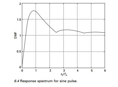
The response spectrum concept is useful in design. A response spectrum is a plot of maximum peak response of the single-degree-of-freedom (SDOF) system oscillator. Different types of shock excitation result in different response spectra which will be discussed in later in this page.

Response to other arbitrary dynamic excitation

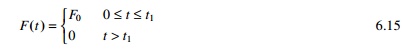
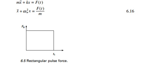
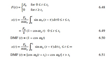
1.Rectangular pulse force

Next let us consider the case of a load F₀ applied instantly to a structure. The force is suddenly removed after a finite time t₁ as shown in Fig. 6.5. Such ais known as force is commonly denoted as rectangular pulse force and t1 duration. When t₁ tends to infinity then the load is a suddenly applied load. The rectangular pulse force is a representative example of an impulsive or shock loading of short duration. Consequently, the response is not significantly affected by the presence of damping in the system. Hence the effect of damping is neglected in the following discussion. The forcing function of the rectangular pulse is defined as

The equation of motion for undamped forced vibration can be written as

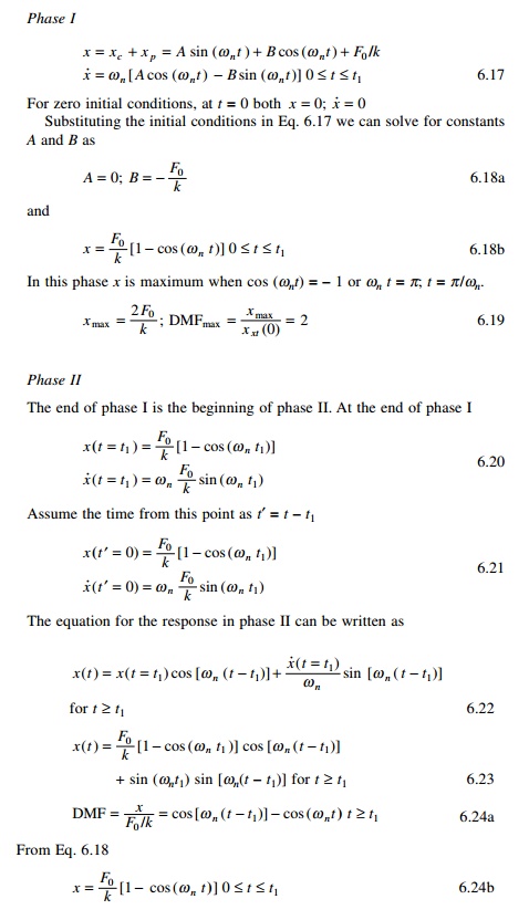
Phase I

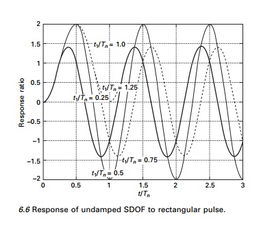
A plot of R(t) vs t/T_n is presented in Fig. 6.6 for several values of t₁/T_n. It is obvious from these plots that during the forced vibration phase, the system oscillates about the static displacement position at its natural period T_n. In the transient phase t tending to t₁, the system oscillates about its original equilibrium position. Examining Fig. 6.5 reveals that maximum displacement for the forced vibration phase = R_max = 2. This can occur when cos(ω t) = �' 1 or ω t = π or 2π/T_n t = π or t/T_n = 0.5 or t must be equal to 0.5 T_n to yield R_max = 2. Thus the maximum displacement response occurs in the forced vibration phase when t₁ > T_n/2.

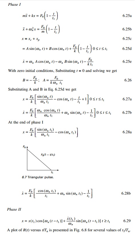
2.Triangular pulse force

A triangular pulse force as shown in Fig. 6.7 is usually employed to simulate a blast. The load F₀ is instantly applied to the structure and decreased linearly over the time duration t₁.

Phase I

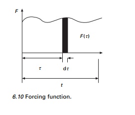
Example 6.1

The shear frame (moment of inertia of the beam is very high) shown in Fig. 6.9 is constructed of a rigid girder and flexible column. The frame supports uniformly distributed load having a total weight of 2.5kN. The frame is

subjected to an impulsive load of triangular pulse as shown in Fig. 6.9 at girder level. Determine the shear in the column.

Duhamel integral

In previous page, it was shown that for any periodic function represented by a trigonometric series, the analysis can be extended by using the principle of superposition to include the solution for a general periodic forcing function.

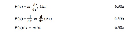
6.5.1     Physical approach

Figure 6.10 shows an arbitrary forcing function in which exciting force is applied at t = 0. The forcing function can be considered as made up of thin strips like F(τ) dτ summed up.

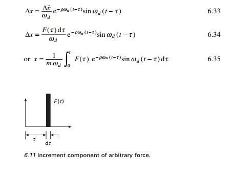
Consider a small strip alone as shown in Fig. 6.11. According to Newton’s second law

F(τ) dτ is called the linear impulse and m ∆x˙ is the momentum. The impulse produces a velocity of ∆x˙ without any displacement. Hence ∆x when t > τ can be written as

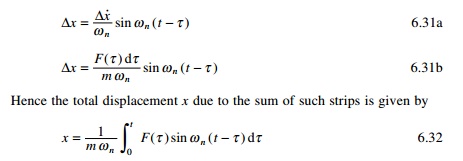
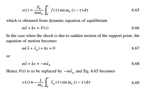
The above integral is known as the Duhamel integral or the convolution integral. For a viscously under-damped system

2.Formal approach

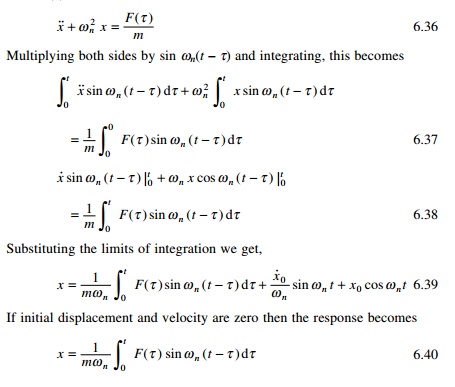
Steps: The differential equation of motion for an undamped system with an exerting force F(τ) is

Multiplying both sides by sin ω_n(t �' τ) and integrating, this becomes

Substituting the limits of integration we get,

If initial displacement and velocity are zero then the response becomes

Response to arbitrary dynamic excitation

To illustrate the application of the Duhamel integral in evaluating the response of an SDOF system to arbitrary excitation, several classical load functions are considered.

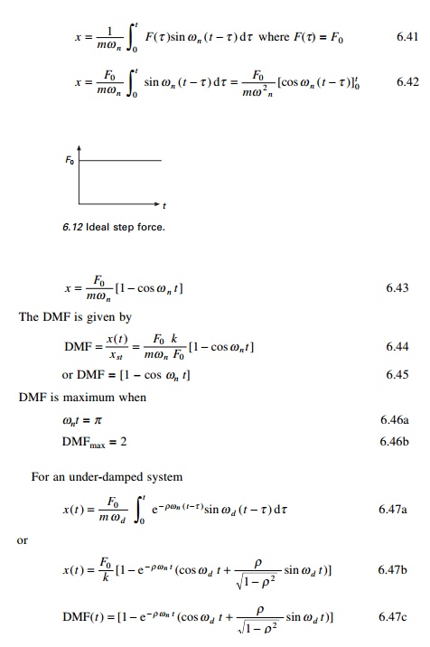
1. Ideal step force

Consider a suddenly applied force of the F₀ that remains constant at all times as shown in Fig. 6.12. For an undamped system

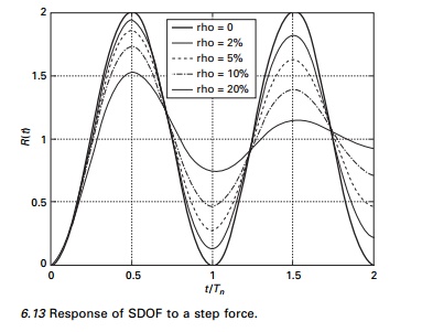
A plot of DMF(t) versus t/T_n is presented in Fig. 6.13 for several levels of damping. DMF(t) = 1 on the response ratio plot corresponds to static displacement position and DMF(t) >1 represents displacement beyond the static displacement position or overshoot. For an undamped system subjected to step force, the resulting response is oscillating motion about the static displacement position with maximum values of DMF_max = 2. In a damped system, the response ratio gradually approaches static values of 1 after a number of cycles of damped oscillation. The maximum overshoot in a damped system as well as the rate of decay of the oscillation about static equilibrium position depends on the damping factor as illustrated in Fig. 6.13.

2.   Program 6.2: MATLAB program to find the response for step force

%program for finding max dynamic response factor for given loading

%define damping ratios for which response is required rho=[0 0.02 0.05 0.1 0.2]

for jj=1:5 zeta=rho(jj);

%assume natural period 1 wn=2*pi;

%assume mass =1

m=1;

% find natural frequency of damped system wd=wn*sqrt(1-zeta^2);

ts=0.002; %sampling period N=1000 % sampling points

%force is defined for ideal step force for n=1:N

t(n)=ts*(n-1); f(n)=1;

end figure(1) plot(t,f)

xlabel(‘ time in secs’) ylabel(‘ force ‘)

title(‘ force definition’) n=[1:N]

g=ts*exp(-(n-1)*zeta*wn*ts).*sin((n-1)*wd*ts)/(m*wd); c0=conv(f,g);

for i=1:N tt(i)=(i-1)*ts;

c1(i)=abs(c0(i)*wn^2); end

figure(2)

plot(tt,c1,‘k’) hold on

end gtext(‘rho=0’) gtext(‘rho=2%’) gtext(‘rho=5%’) gtext(‘rho=10%’) gtext(‘rho=20%’) xlabel(‘ t/Tn’); ylabel(‘ R(t)’)

title(‘ Response of SDOF to ideal step force’)

3 Rectangular pulse force

Let us consider the case of load F₀ applied instantly to a structure for a finite time duration of t₁ known as rectangular pulse.

Undamped system

For an under-damped system similar to Eq. 6.47, the response can be derived.

Several plots of DMF(t) as a function of t/T_n for several values of t₁/T_n are presented in Fig. 6.14. It is seen that DMF_max = 2 which can occur at cos ω_n t = �'1.

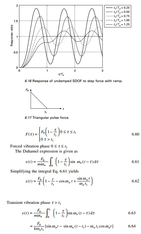
4     Step force with ramp

Consider a force which is applied over a finite time t₁. Such a forcing function is called a ramp function and is shown in Fig. 6.15. The dynamic response is significantly affected by t₁/T_n.

The Duhamel integral for the loading in the time interval 0 ≤ t ≤ t₁

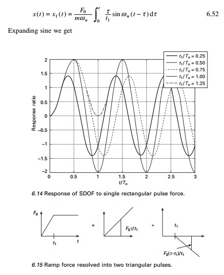
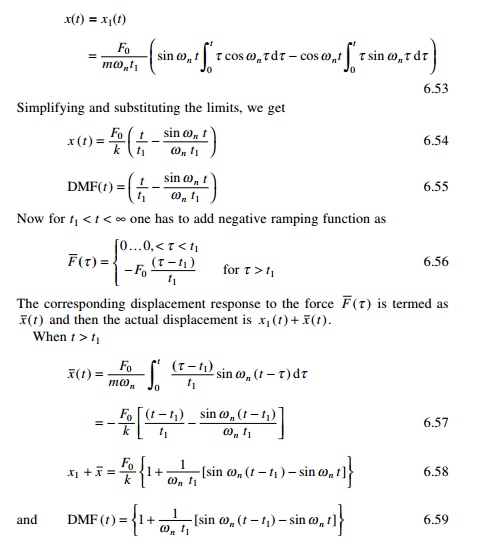
Figure 6.16 shows the plot of response ratio values versus t/T_n for several ratios of t₁/T_n. These plots indicate that as t₁ approaches zero (t₁/T_n << 1) the response approaches that of an ideal step function. Dynamic effects can be ignored for ramp forces if t₁/T_n > 3.0.

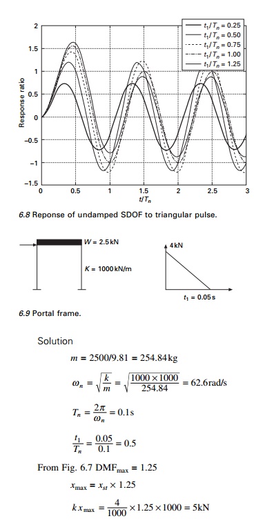
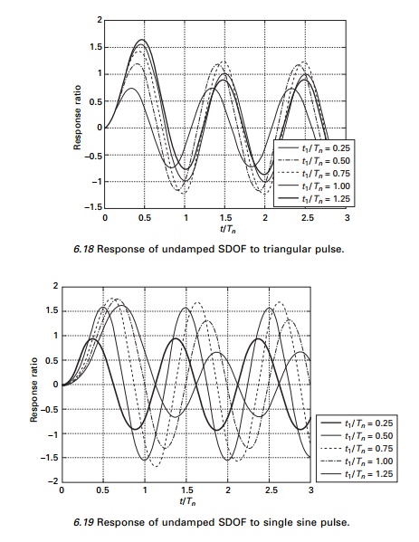
6.6.5 Triangular pulse force

A load function often employed to simulate blast is the triangular pulse shown in Fig. 6.17. The load F₀ is instantly applied to the structure and decreases linearly over the time duration t₁.

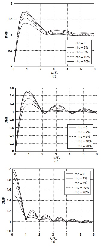
Once the Duhamel integral has been evaluated for a specific forcing function, the result may be used to evaluate response of any SDOF system to that particular type of loading. Figure 6.18 depicts the plot of response ratio versus t/T_n for triangular loading for several values of t₁/T_n, the overshoot becomes less with smaller oscillations above the static displacement position. Similarly such curves are drawn for step single sine pulse and double triangle, in Figs 6.19 and 6.20 respectively.

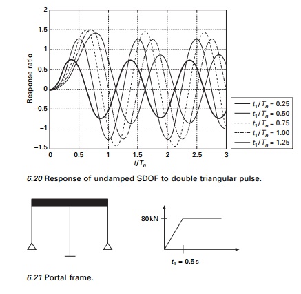
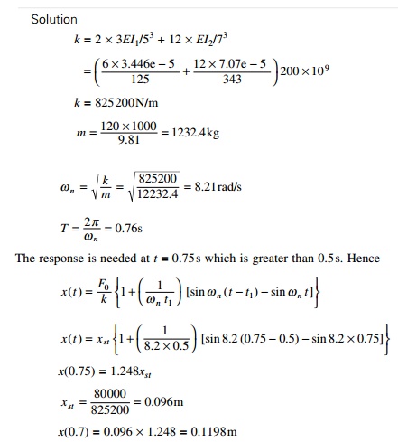
Example 6.2

The shear frame shown in Fig. 6.21 is constructed of rigid girder and flexible columns. The frame supports uniformly distributed load of total weight of 120kN and the frame is subjected to step force with a ramp as shown in Fig. 6.21 at the girder level. Determine the horizontal displacement at t = 0.75s. E = 200 GPa and damping can be assumed as zero. Moment of inertia of end columns and centre column are 3.4465e^�'5mm⁴ and 7.07e^�'5mm⁴ respectively.

The Duhamel method is a closed form procedure for calculating a system response to arbitrary dynamic excitation. But evaluation of the integral is cumbersome as evidenced in previous sections. But with the MATLAB and MATHEMATICA packages these convolution integrals may be evaluated quite easily. It is not possible to apply a closed form procedure for earthquake ground motion since ground motion recordings are in digitized form. In such cases a numerical procedure is resorted to.

Response spectrum

A shock represents a sudden application of force or other form of disruption which results in a transient response of a system. The maximum value of the response is a good measure of the severity of the shock and is of course dependent upon dynamic characteristics of the system. In order to categorize all types of shock excitation an SDOF system oscillator is chosen as the standard.

The response spectrum concept is useful in design. A response spectrum is a plot of maximum peak response of the SDOF system oscillator. Different types of shock excitation result in different response spectra. It is possible to have similar response spectra for two different shock excitation. In spite of this limitation, the response spectrum is a useful concept that is extensively used.

Consider the excited force function as F(τ) = F₀f (τ) and the response for SDOF of an undamped system as given by

The inner product given in the integral is f(τ) sin ω_n(t �' τ) and the integral is known as the convolution integral. MATLAB can calculate a convolution integral very easily.

Program 6.3: MATLAB program to find the response spectrum for any load pulse

%program for finding max dynamic response factor for given loading

%define damping ratios for which response is required rho=[0 0.02 0.05 0.1 0.2]

for jj=1:5 zeta=rho(jj);

%define the fac=td/Tn= duration of loading / natural period for ii=1:193

fac(ii)=0.03125*(ii-1);

td=0.1; %period of forcing function

%natual frequency of the system

wn=fac(ii)*2*pi/td;

%assume mass =1 m=1;

%find natural frequency of damped system wd=wn*sqrt(1-zeta^2);

ts=0.002; %sampling period N=1000 % sampling points load=1

%force is defined for rectangular pulse

for n=1:N t(n)=ts*(n-1); if n>td/ts+1

f(n)=0;

else

f(n)=1;

end end %load=2

%force is defined for triangular load %for n=1:N

%t(n)=ts*(n-1);

%if n>td/ts+1

%f(n)=0;

%else

%f(n)=1-t(n)/td;

%end

%end

%load=3

%force is defined for sinusoidal loading

%defining force

%for n=1:N

%t(n)=ts*(n-1);

%if n>td/ts+1

%f(n)=0;

%else

%f(n)=sin(pi*t(n)/td);

%end

%end

%load=4;

%force is defined for double triangular load

%for n=1:N

%t(n)=ts*(n-1);

%if n<=(td/2)/ts+1

%f(n)=2.0*(n-1)*ts/td;

%else

%f(n)=2.0*(1-(n-1)*ts/td);

%end

%if n>td/ts+1;

%f(n)=0; end

%end

%load=5

force is defined as ramp loading

%for n=1:N

%t(n)=ts*(n-1);

%if n>td/ts+1

%f(n)=1;

%else

%f(n)=t(n)/td;

%end

%end

figure(1)

plot(t,f)

xlabel(‘ time in secs’) ylabel(‘ force ’)

title(‘ force definition’) n=[1:N]

g=ts*exp(-(n-1)*zeta*wn*ts).*sin((n-1)*wd*ts)/(m*wd); c0=conv(f,g);

for i=1:N tt(i)=(i-1)*ts; c1(i)=c0(i)*wn^2;

end dmf(ii)=max(abs(c1)); end

if load<4 dmf(1)=0

else end

figure(2)

plot(fac,dmf,‘k’) hold on

end gtext(‘rho=0’) gtext(‘rho=2%’) gtext(‘rho=5%’) gtext(‘rho=10%’) gtext(‘rho=20%’) xlabel(‘ td/Tn’); ylabel(‘ DMF’)

title(‘ Response spectrum for the given loading’)

The responses spectrum for (a) rectangular pulse, (b) triangular pulse, (c) sine pulse, (d) double triangle pulse and (e) step ramp loadings are shown in Fig. 6.22.

Example 6.3

Determine the maximum horizontal displacement of structural frame when subjected to ramp loading as given in Example 6.2.

DMF_max = 1.5

x_max = 1.5 �- 0.096 = 0.144m

The construction of response spectrum can be greatly facilitated through numerical evaluation techniques. The construction of a response spectrum by numerical integration is addressed in later chapters. Once constructed, the response spectrum offers the design engineer an opportunity to evaluate the response of a wide frequency range of structures to a specific input.

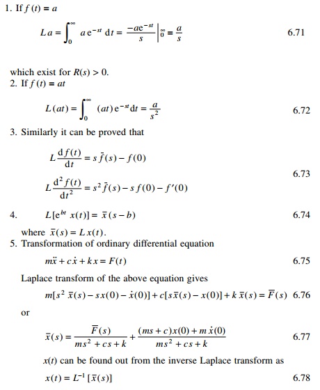
Laplace transform

The Laplace transform method of solving the differential equation provides a complete solution, yielding both transient and forced vibrations. Here in we give a brief introduction of the theory and illustrate with some examples.

If f (t) is a function of t for t > 0 its Laplace transform f (s) is defined as

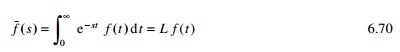
where ‘s’ is a complex variable. For the real part of s > 0 the integral exists provided f (t) is absolutely integrable function in the time interval 0 to infinity.

For Laplace transform of simpler expressions, the reader may consult any mathematics handbook or one can use the MATHEMATICA package to obtain both Laplace transform and inverse Laplace transform.

Example 6.4

Write a MATHEMATICA program to obtain the motion of the mass subjected to initial conditions. There is no external forcing function. The SDOF system is shown in Fig. 6.23; m = 4kg, K = 10N/m; c = 6Ns/m and at t = 0 x (0) = 0.1m and x˙ (0) = 0.16m/s.

Taking inverse transform of the above equation, we get x(t) which is given in the MATHEMATICA program.

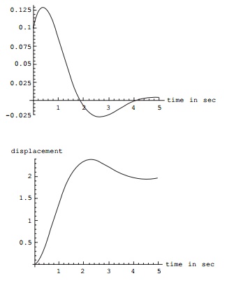
Example 6.5

For the same problem, when 20N force (step input) is applied and the system is at rest initially.

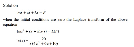
Taking inverse transform we get x(t) which is given in MATHEMATICA program.

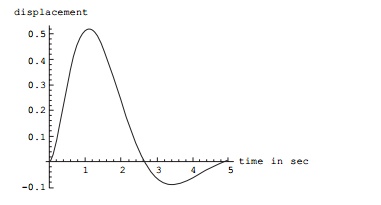
Example 6.6

When F(t) = 20e^�'2t.

Solution

Program 6.4: MATHEMATICA program for Laplace transform method

f=InverseLaplaceTransform[(.1 *s+0.31)/

(s^2+1.5*s+2.5),s,t]

E^((-0.75 - 1.3919410907075054*I)*t)* (0.05000000000000001 + 0.08441449195258423*I + (0.05 -0.08441449195258421*I)* E^(2.7838821814150108*I*t)) f

E^((-0.75 - 1.3919410907075054*I)*t) *(0.05000000000000001 + 0.08441449195258423*I + (0.05 - 0.08441449195258421*I)*E^(2.7838821814150108*I*t)) Plot[f,{t,0,5},AxesLabel�'{“time in sec”, “displacement”},PlotStyle�'{Thickness[0.008]}]

g=InverseLaplaceTransform[(20)/(s*(4*s^2+6*s+10)),s,t]

2/31*(31 - (31*Cos[(Sqrt[31]*t)/4])/E^((3*t)/4) - (3*Sqrt[31]*Sin[(Sqrt[31]*t)/4])/E^((3*t)/4))

Plot[g,{t,0,5},AxesLabelÆ{“time in sec”, “displacement”},PlotStyleÆ{Thickness[0.008]}]

h=InverseLaplaceTransform[(20)/

((s+3)*(4*s^2+6*s+10)),s,t]

(5/217*(31 - 31*E^((9*t)/4)*Cos[(Sqrt[31]*t)/4] +

9*Sqrt[31]*E^((9*t)/4)*Sin[(Sqrt[31]*t)/4]))/E^(3*t)

Plot[h,{t,0,5},AxesLabel�'{“time in sec”, “displacement”},PlotStyle�'{Thickness[0.008]}]

Summary

In this chapter, the response spectrum is constructed only for certain loads such as rectangular, triangular, double triangle, sine and ramp pulses. For any other general pulses, the numerical technique as addressed in Chapter 7 should be used. Once constructed, the response spectrum offers the design engineer the opportunity to evaluate the maximum response of a wide frequency range of structures to a specific input. Application of the response spectrum will follow in later chapters for earthquake loading.