Chapter:
Dynamic response of structures using numerical methods
Dynamic
response of structures using numerical methods
Abstract: There are
two basic approaches to numerically evaluate the dynamic response. The
first approach is numerical interpolation of the excitation and the second is
numerical integration of the equation of motion. Both approaches are applicable
to linear systems but the second approach is related to non-linear systems. In
this chapter, various numerical techniques based on interpolation, finite
difference equation and assumed acceleration are employed to arrive at the
dynamic response due to force and base excitation.
Key words: time stepping, time history,
central difference, explicit method, Runge-Kutta method, Newmark’s method,
Wilson-θ method.
Introduction
It was clearly demonstrated in earlier
chapters that analytical or closed form solution of the Duhamel integral
can be quite cumbersome even for relatively simple excitation problems.
Moreover, the exciting force such as an earthquake ground record cannot be
expressed by a single mathematical expression, such as the analytical solution
of the Duhamel integral procedure. Hence to solve practical problems, numerical
evaluation techniques must be employed to arrive at the dynamic response.
To evaluate dynamic response
problem there are two approaches, the first of which has two parts:
1. Numerical
interpolation of the excitation
2. Numerical
integration and Duhamel integral.
The other approach is derived by integration of the equation
of motion
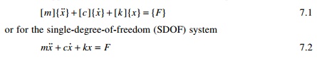
or for the single-degree-of-freedom (SDOF) system
Both the above approaches are applicable to linear systems,
but only the second approach is valid for non-linear systems.
Time stepping methods
Assume an inelastic equation to be solved as
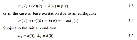
Subject to the initial condition
Usually the system is assumed to have a linear damping, but
other forms of damping such as nonlinear damping should be considered. The
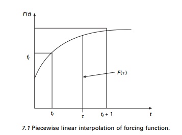
applied force F(t) is defined at discrete time intervals and the
time increment (see Fig. 7.1)

may be assumed as constant, although this is not necessary. If
the response is determined at the time ti, is called ith
step displacement; velocity and acceleration at the ith step are denoted
by u i , u˙ i , u˙˙i
respectively. The displacement, velocity and acceleration are assumed to be
known, satisfying Eq. 7.3 as

The third term on the left has solution gives the resisting
force at time ti as fsi and for linear elastic
system but would depend on the prior history of displacement and the
velocity at time �'i’ if the system were inelastic. We have to discuss
the numerical procedure, to determine the response quantities
u i + 1 , u˙
i + 1 , u˙˙i
+1 as i +
1th step. Similar to Eq. 7.7, at (i + 1)th step the dynamic
equilibrium equation is written as

if the numerical procedure is
applied successively with i = 0, 1, 2,É. The time stepping procedure
gives the desired response at all times with the known initial conditions u0
and u˙0 .
The time stepping procedure is
not an exact procedure. The characteristics of any numerical procedure that
converges to a correct answer are as follows:
• Convergence
- if the time step is recorded, the procedure should converge to an exact
solution.
• The
procedure should be stable in the presence of numerical rounding errors.
The procedure should provide results close enough to the exact
solution.
Types of time stepping
method
There are three types of time stepping method:
1. Methods
based on the interpolation of the excitation function (See Section 7.3.1).
2. Methods
based on finite difference expressions for the velocity and acceleration (See
Section 7.3.3).
3. Methods
based on assumed variation of acceleration (See Section 7.3.5).
1 Interpolation of the excitation
Duhamel integral expression for the damped and undamped SDOF
system to arbitrary excitation can be solved using numerical quadrature
techniques such as Simpson’s method, trapezoid method or Gauss rule.
It is generally more convenient to interpolate the excitation function F(t)
as (see Fig. 7.1)
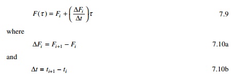
F(τ) is
known as interpolated force and τ varies from 0 to ∆t. Hence differential equation of noted for an
undamped SDOF system becomes
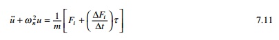
The solution of Eq. 7.11 of the
sum of the homogeneous and particular solutions on the time interval 0 ≤ τ ≤ ∆t. The
homogeneous part of the solution is evaluated for initial condition of
displacement ui and velocity u˙i
at τ = 0.
The particular solution consists of two parts: (1) the
response to an real step for a magnitude of Fi ; and (2) the
response to a ramp function by (∆Fi/∆t)τ. Hence
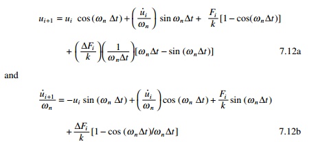
tion 7.12a and 7.12b are the
recurrence formulae for computing displacement ui+1
and velocity u˙i +1 at time ti+1.
Recurrence formulae for a
displacement and velocity under-damped system may be derived in the same
manner. A simpler and more convenient representation of the recurrence formulae
simplified by Eq. 7.12a and 7.12b are
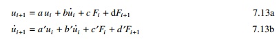
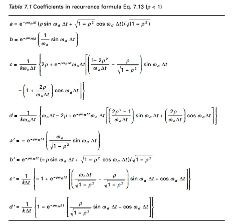
Equation 7.13a and 7.13b are the
recurrence formulae for ρ < 1.
The coefficients given in Table 7.1 depend on ωn, k and ρ and time interval ∆t. In
practice ∆t should
be sufficiently small to closely approximate the excitation force and also to
render results at the required time intervals. The practice to select ∆t ≤ T/10 where
T is the natural period of the structure. This is to ensure that the important
peaks of structural response are not omitted. As long as ∆t is constant, the recurrence formulae
coefficients need to be calculated once.
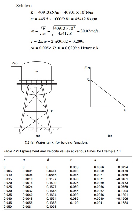
Example 7.1
The water tank shown in Fig.7. 2a is subjected to the blast
loading illustrated in Fig 7.2b. Write a computer program in MATLAB to
numerically evaluate
the dynamic response of the tower
by interpolation of the excitation. Plot the displacement u(t)
and velocity u˙ (t ) response in time interval 0 ≤ t < 0.5s. Assume W =
445.5kN, k = 40913kN/m, ρ = 0.05; F0 = 445.5kN, td
= 0.05s. Use the step size as 0.005s.
Calculate natural period.
The constants are calculated as
a = 0.9888 a′ = -4.4542
b = 0.0049 b′ = 0.9740
c = 1.82 e-10 c′ = 5.4196e-08
d = 9.1305e-011 d′ = 5.467e-08
Using the recurrence formulae u
and u˙ can be calculated as shown in Table 7.2.
The displacement time history and the velocity time history
are plotted as shown in Fig. 7.3 and the program is given below.
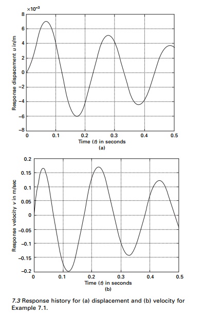
Response history for (a) displacement and (b) velocity
for Example 7.1.
Program 7.1: MATLAB program for dynamic response of SDOF
using recurrence formulae
%*********************************************************** %
DYNAMIC RESPONSE DUE TO EXTERNAL LOAD USING WILSON RECURRENCE FORMULA
%
**********************************************************
m=45412.8;
k=40913000;
wn=sqrt(k/m)
r=0.05;
u(1)=0;
v(1)=0;
tt=.50;
n=100;
n1=n+1
dt=tt/n;
td=.05;
jk=td/dt;
for
m=1:n1
p(m)=0.0;
end
t=-dt
% **********************************************************
% ANY
EXTERNAL LOADING VARIATION MUST BE DEFINED HERE
%
**********************************************************
for
m=1:jk+1;
t=t+dt;
p(m)=445500*(td-t)/td;
end
wd=wn*sqrt(1-r^2);
a=exp(-r*wn*dt)*(r*sin(wd*dt)/sqrt(1-r^2)+cos(wd*dt));
b=exp(-r*wn*dt)*(sin(wd*dt))/wd;
c2=((1-2*r^2)/(wd*dt)-r/sqrt(1-r^2))*sin(wd*dt)-(1+2*r/(wn*dt))*cos(wd*dt);
c=(1/k)*(2*r/(wn*dt)+exp(-r*wn*dt)*(c2));
d 2 = e x p ( - r * w n * d t ) * ( ( 2 . 0 * r ^ 2 - 1 ) / (
w d * d t ) * s i n ( w d . * d t ) + 2 . 0 * r /
(wn*dt)*cos(wd*dt));
d=(1/k)*(1-2.0*r/(wn*dt)+d2);
ad=-exp(-r*wn*dt)*wn*sin(wd*dt)/(sqrt(1-r^2));
bd=exp(-r*wn*dt)*(cos(wd*dt)-r*sin(wd*dt)/sqrt(1-r^2));
c 1 = e x p ( - r * w n * d t ) * ( ( w n / s q r t ( 1 - r ^
2 ) + r / ( d t * s q r t ( 1 - r^2)))*sin(wd*dt)+cos(wd*dt)/dt);
cd=(1/k)*(-1/dt+c1);
d1=exp(-r*wn*dt)*(r*sin(wd*dt)/sqrt(1-r^2)+cos(wd*dt)); dd=(1/(k*dt))*(1-d1);
for m=2:n1 u(m)=a*u(m-1)+b*v(m-1)+c*p(m-1)+d*p(m);
v(m)=ad*u(m-1)+bd*v(m-1)+cd*p(m-1)+dd*p(m);
end
for m=1:n1 s(m)=(m-1)*dt
end figure(1);
plot(s,u,�'k’);
xlabel(�'
time (t) in seconds’)
ylabel(�' Response displacement u in m’) title(�' dynamic
response’)
figure(2);
plot(s,v,�'k’);
xlabel(�'
time (t) in seconds’)
ylabel(�' Response velocity v in m/sec’) title(�' dynamic
response’)
3 Direct
integration of equation of motion
In direct integration, the
equation of motion is integrated using a step-by-step procedure. It has two
fundamental concepts: (1) the equation of motion is satisfied at only discrete
time intervals ∆t and (2)
for any time t, the variation of displacements, velocity and
acceleration with each time interval ∆t is assumed.
Consider the SDOF system

It is assumed that displacement velocity and acceleration at
time t = 0 are given as u0, u˙ 0,
u˙˙0 respectively. Algorithms can be derived to calculate
the solution at some time t + ∆t based upon the solution at time ‘t’.
Several commonly based direct integration methods are presented below.
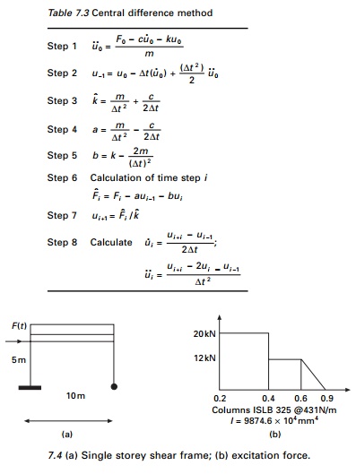
Central difference method
This method is based on finite difference approximation of the
time derivations of displacements (velocity and acceleration). Taking a
constant time step ∆t
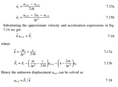
The above method uses equilibrium
condition at time i but does not satisfy equilibrium condition at i
+ 1.
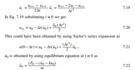
In Eq. 7.17b it is observed that known displacements of ui,
ui-1 are used to interpolate ui+1.
Such methods are called explicit methods. In Eq. 7.17b, it is observed
that known displacements of ui, ui-1
are required to determine ui+1. Thus u0,
u-1 are required to determine u1.
This is not a constraint for SDOF
systems because a much smaller time step is chosen for better accuracy. The
steps taken in the central difference method are given in Table 7.3.
Example 7.2
A single story shear frame shown in Fig. 7.4a is subjected to
arbitrary excitation force specified in Fig. 7.4b. The rigid girder supports a
load of 25.57kN/m.
Assume the columns bend about
their major axis and neglect their mass, and assuming damping factor of ρ = 0.02 for steel structures, E
= 200GPa. Write a computer program for the central difference method to
evaluate dynamic response for the frame. Plot displacement u(t),
velocity v(t) and acceleration a(t) in the interval
0 ≤ t ≤ 5s.
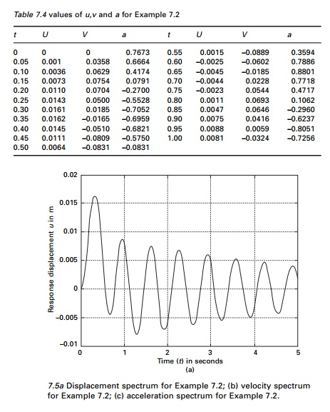
Solution
(a) The total
load on the beam = 25.57 �- 10 = 255.7kN
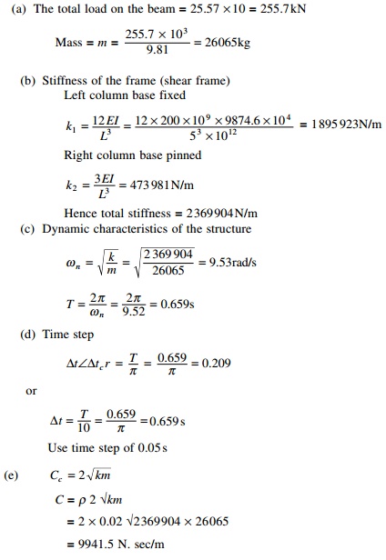
Table 7.4 gives the displacement, velocity and acceleration up
to 1s.
The displacement, velocity and acceleration response are shown
in Fig. 7.5. The computer program in MATLAB is given below.
Program 7.2: MATLAB program for
dynamic response of SDOF using central difference method
%**********************************************************
%DYNAMIC
RESPONSE USING CENTRAL DIFFERENCE METHOD
%**********************************************************
ma=26065;
k=2369904.0;
wn=sqrt(k/ma)
r=0.02;
c=2.0*r*sqrt(k*ma)
u(1)=0;
v(1)=0;
tt=5;
n=100;

n1=n+1
dt=tt/n;
td=.9;
jk=td/dt;
%*********************************************************** %
LOADING IS DEFINED HERE
%***********************************************************
for m=1:n1
p(m)=0.0; end
t=-dt
for m=1:8; t=t+dt; p(m)=20000;
end p(9)=16000.0 for m=10:12 t=t+dt
p(m)=12000.0 end
for m=13:19 t=t+dt
p(m)=12000.0*(1-(t-0.6)/.3) end
an(1)=(p(1)-c*v(1)-k*u(1))/ma up=u(1)-dt*v(1)+dt*dt*an(1)/2
kh=ma/(dt*dt)+c/(2.0*dt) a=ma/(dt*dt)-c/(2.0*dt) b=k-2.0*ma/(dt*dt)
f(1)=p(1)-a*up-b*u(1) u(2)=f(1)/kh
for m=2:n1 f(m)=p(m)-a*u(m-1)-b*u(m)
u(m+1)=f(m)/kh
end v(1)=(u(2)-up)/(2.0*dt) for
m=2:n1
v(m)=(u(m+1)-u(m-1))/(2.0*dt)
an(m)=(u(m+1)-2.0*u(m)+u(m-1))/(dt*dt) end
n1p=n1+1 for m=1:n1p
s(m)=(m-1)*dt end
for m=1:n1 x(m)=(m-1)*dt end
figure(1);
plot(s,u,’k’);
xlabel(‘
time (t) in seconds’)
ylabel(‘ Response displacement u in m’) title(‘ dynamic
response’)
figure(2);
plot(x,v,’k’);
xlabel(‘
time (t) in seconds’)
ylabel(‘ Response velocity v in m/sec’) title(‘ dynamic
response’)
figure(3);
plot(x,an,’k’);
xlabel(‘
time (t) in seconds’)
ylabel(‘ Response acceleration a in m/sq.sec’) title(‘ dynamic
response’)
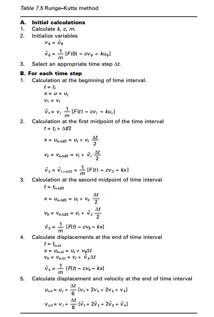
4.Single step methods
Runge�'Kutta method
These methods are classified as single step since they require
knowledge of only xi to determine xi+1.
Hence the methods are called self-starting as they require no special starting
procedure unlike the central difference method. The Runge-Kutta method of order
4 is usually applied in practice. Consider the differential equation of motion
for a single degree of freedom as
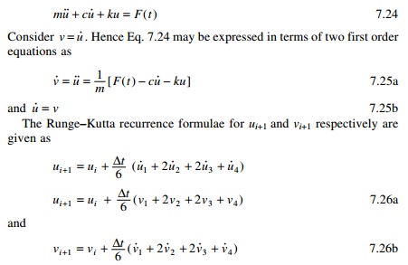
Equations 7.26a and 7.26b represent an averaging of the
velocity and acceleration by Simpson’s rule within the time interval ∆t. The
fourth order Runge-Kutta method is summarized in Table 7.5.
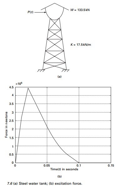
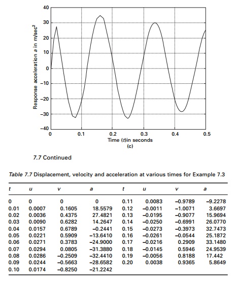
Example 7.3
A steel water tank shown in Fig.
7.6a is analysed as an SDOF system having a mass on top of cantilever which
acts as a spring and dashpot for damping. A blast load of P(t) is
applied as shown in Fig. 7.6b. The values of the force are given in Table 7.6.
Draw displacement, velocity and acceleration responses up to 0.5s. The damping
for steel may be assumed to be 2% of critical damping.
Solution
Given
W = 133.5kN
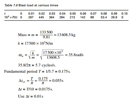
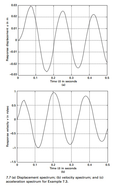
Figure 7.7 shows the displacement, velocity and acceleration
response for the tank. The values are given in Table 7.7 and the program is
given below.
%********************************************************************
% DYNAMIC RESPONSE DUE TO EXTERNAL LOADING RUNGE KUTTA METHOD %********************************************************************
ma=13608.5;
k=17500000;
wn=sqrt(k/ma)
r=0.02;
c=2.0*r*sqrt(k*ma)
u(1)=0;
v(1)=0;
tt=.5;
n=50;
n1=n+1
dt=tt/n;
td=.1;
jk=td/dt;
%**************************************************************
% EXTERNAL LOADING IS DEFINED HERE
%************************************************************** for m=1:n1
p(m)=0.0; end p(2)=267000.0 p(3)=445000.0 p(4)=364000.0
p(5)=284000.0 p(6)=213000.0 p(7)=142000.0 p(8)=89000.0
p(9)=53400.0
p(10)=26700.0
an(1)=(p(1)-c*v(1)-k*u(1))/ma t=0.0
for i=2:n1 ui=u(i-1) vi=v(i-1)
ai=an(i-1) d(1)=vi q(1)=ai for j=2:3 l=0.5
x=ui+l*dt*d(j-1)
d(j)=vi+l*dt*q(j-1) q(j)=(p(i)-c*d(j)-k*x)/ma end
j=4
l=1 x=ui+l*dt*d(j-1)
d(j)=vi+l*dt*q(j-1)
q(j)=(p(i)-c*d(j)-k*x)/ma
u(i)=u(i-1)+dt*(d(1)+2.0*d(2)+2.0*d(3)+d(4))/6.0
v(i)=v(i-1)+dt*(q(1)+2.0*q(2)+2.0*q(3)+q(4))/6.0 an(i)=(p(i)-c*v(i)-k*u(i))/ma
end
for i=1:n1 s(i)=(i-1)*dt end
figure(1);
plot(s,u,’k’);
xlabel(‘
time (t) in seconds’)
ylabel(‘ Response displacement u in m’) title(‘ dynamic
response’)
figure(2);
plot(s,v,’k’);
xlabel(‘
time (t) in seconds’)
ylabel(‘ Response velocity v in m/sec’) title(‘ dynamic
response’)
figure(3);
plot(s,an,’k’);
xlabel(‘
time (t) in seconds’)
ylabel(‘ Response acceleration a in m/sec’) title(‘ dynamic
response’)
figure(4);
plot(s,p,’k’)
xlabel(‘ time (t) in seconds’)
ylabel(‘ force in Newtons’) title(‘ Excitation Force’)
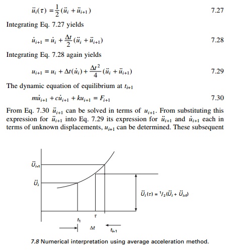
7.3.5 Assumed
acceleration methods
Average acceleration method
It is assumed that with a small increment of time ∆t, the
acceleration is the average value of the acceleration at the beginning of the
interval u˙˙i and the acceleration at the end
of the interval u˙˙i +1 as
illustrated in Fig. 7.8. Hence acceleration at the some time τ between ti and ti+1
can be expressed as
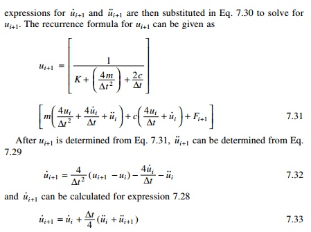
A computational algorithm can be developed in terms of
incremental quantities for applied load ∆Fi for displacement ∆ui for velocity
∆u˙i and for
acceleration ∆u˙˙i quantities
as
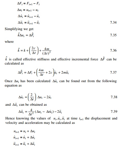
Even though this kind of
incremental form is not necessary for linear systems, it is required for
nonlinear systems and with non-proportional damping which we will see in a
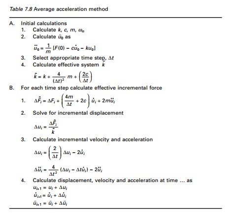
later chapter. Table 7.8 gives a step-by-step solution using the average
acceleration method (incremental form).
Table 7.8 Average acceleration
method
It can be proved that the average
acceleration method or constant acceleration method just discussed is
equivalent to the trapezoidal rule. It is also a special form of the Newmark
method which will be discussed later.
Example 7.4
The shear frame shown in Fig.
7.9a is subjected to the exponential pulse force shown in Fig 7.9b. Write a
computer program for the average acceleration method (incremental formulation)
to evaluate the dynamic response of the frame. Plot the time histories for
displacement u(t), velocity u˙ (t ) and
acceleration u˙˙(t ) in the time interval 0-3s. Assume E
= 200 GPa, W = 1079.1kN, ρ = 0.07, F0 = 450kN and td
= 0.75s and use a time step ∆t of
0.01s.
Solution
Given
I for ISWB
600 @1337 = 106 198.5e4mm4
Mass = m
= 110 000 kg
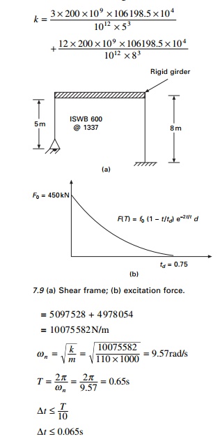
∆t ≤ 0.065s
We use ∆t = 0.01s.
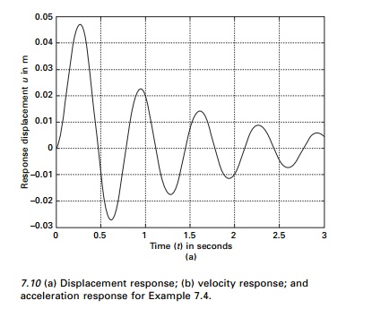
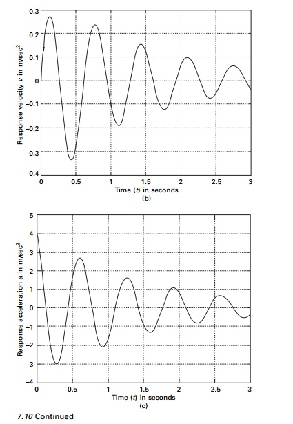
The displacement velocity and
acceleration response are shown in Fig. 7.10 and the values are given in Table
7.9. The program using MATLAB for constant acceleration method is given below.
Program 7.4: MATLAB program for
dynamic response by constant acceleration method
% Response by constant acceleration method. ma=110000;
k=10075582;
wn=sqrt(k/ma)
r=0.07;
c=2.0*r*sqrt(k*ma)
u(1)=0;
v(1)=0;
tt=3;
n=300;
n1=n+1
dt=tt/n;
td=.75;
jk=td/dt; for m=1:n1
p(m)=0.0; end jk1=jk+1 for
n=1:jk1 t=(n-1)*dt
p(n)=450000*(1-t/td)*exp(-2.0*t/td)
end
an(1)=(p(1)-c*v(1)-k*u(1))/ma
kh=k+4.0*ma/(dt*dt)+2.0*c/dt for i=1:n1
s(i)=(i-1)*dt end
for i=2:n1 ww=p(i)-p(i-1)+(4.0*ma/dt+2.0*c)*v(i-1)+2.0*ma*an(i-1)
xx=ww/kh
yy=(2/dt)*xx-2.0*v(i-1)
zz=(4.0/(dt*dt))*(xx-dt*v(i-1))-2.0*an(i-1) u(i)=u(i-1)+xx
v(i)=v(i-1)+yy an(i)=an(i-1)+zz
end
figure(1);
plot(s,u);
xlabel(‘
time (t) in seconds’)
ylabel(‘ Response displacement u in m’) title(‘ dynamic
response’)
figure(2);
plot(s,v);
xlabel(‘
time (t) in seconds’)
ylabel(‘ Response velocity v in m/sec’) title(‘ dynamic
response’)
figure(3);
plot(s,an);
xlabel(‘
time (t) in seconds’)
ylabel(‘ Response acceleration a in m/sec’) title(‘ dynamic
response’)
figure(4);
plot(s,p)
xlabel(‘ time (t) in seconds’)
ylabel(‘ force in Newtons’) title(‘ Excitation Force’)
6.Assumed acceleration
method (linear variation)
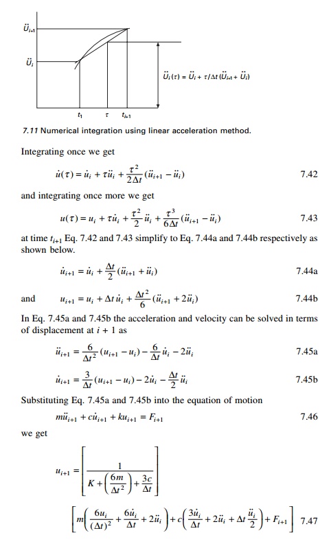
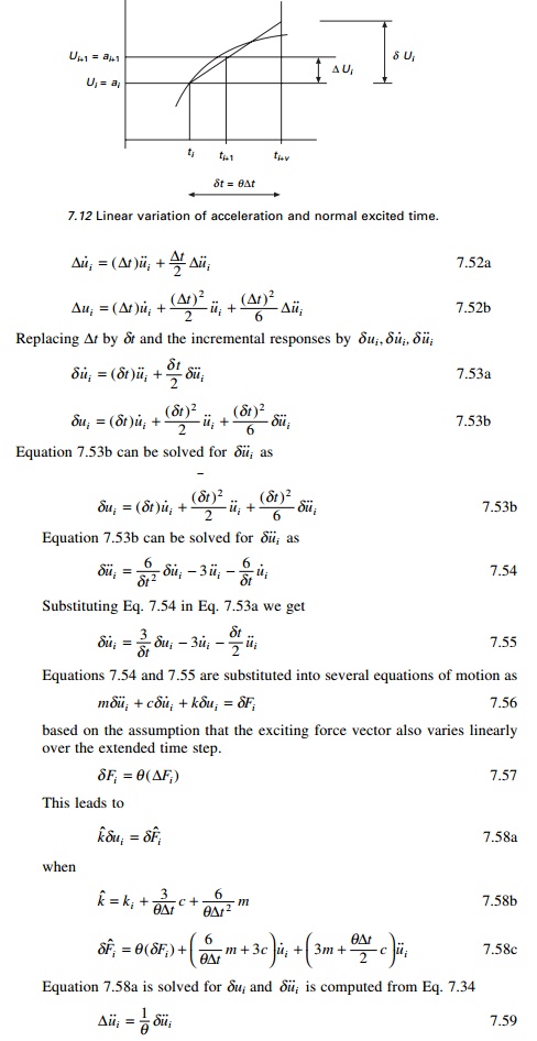
Linear acceleration method
In this method a linear variation of acceleration from time ti
to ti+1 is assumed as illustrated in Fig 7.11. Let
τ denote the time within the
interval ti and ti+1 such that 0
≤ τ ≤ ∆t (see
Fig. 7.11). Then acceleration at time τ
is expressed as
After determining ui+1
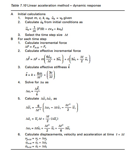
Eq. 7.45a and 7.45b may be used to determine velocity u˙i+1 and acceleration u˙˙i+1 . The above algorithm is for
total formulation. However this algorithm can be modified for incremental
formulation as shown in Table 7.10.
The displacement velocity and acceleration are almost the same
as in the average acceleration method and the response curve is exactly the
same as in Fig. 7.10. The program for linear acceleration method in MATLAB is
given below.
Program 7.5: MATLAB program for
dynamic response by linear acceleration method
![]()
% Linear Acceleration Method. %*******************************
ma=110000;
k=10075582;
wn=sqrt(k/ma)
r=0.07;
c=2.0*r*sqrt(k*ma)
u(1)=0;
v(1)=0;
tt=3;
n=300;
n1=n+1
dt=tt/n;
td=.75;
jk=td/dt; for m=1:n1
p(m)=0.0; end jk1=jk+1 for
n=1:jk1 t=(n-1)*dt
p(n)=450000*(1-t/td)*exp(-2.0*t/td)
end
an(1)=(p(1)-c*v(1)-k*u(1))/ma
kh=k+6.0*ma/(dt*dt)+3.0*c/dt for i=1:n1
s(i)=(i-1)*dt end
for i=2:n1
ww=p(i)-p(i-1)+ma*(6.0*v(i-1)/dt+3.0*an(i-1))+c*(3.0*v(i-1)+dt*an(i-1)/2)
xx=ww/kh
zz=(6.0/(dt*dt))*(xx-dt*v(i-1)-dt*dt*an(i-1)/2)
yy=dt*an(i-1)+dt*zz/2.0 vv=v(i-1)*dt+(dt*dt)*(3.0*an(i-1)+zz)/6.0
v(i)=v(i-1)+yy
an(i)=an(i-1)+zz u(i)=u(i-1)+vv
end
figure(1);
plot(s,u);
xlabel(‘
time (t) in seconds’)
ylabel(‘ Response displacement u in m’) title(‘ dynamic response’)
figure(2);
plot(s,v);
xlabel(‘
time (t) in seconds’)
ylabel(‘ Response velocity v in m/sec’) title(‘ dynamic
response’)
figure(3);
plot(s,an);
xlabel(‘
time (t) in seconds’)
ylabel(‘ Response acceleration a in m/sec’)
title(‘ dynamic response’)
figure(4);
plot(s,p)
xlabel(‘ time (t) in seconds’)
ylabel(‘ force in Newtons’) title(‘ Excitation Force’)
7.Stepping methods
Newmark’s method
In 1959, N.M. Newmark developed a time stepping method
based on the following equations:
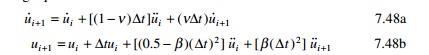
The parameter β and γ define the variation of
acceleration over a time step and determine the stability and accuracy
characteristics of the method. Usually
γ is
selected as 1/2 and
16 ≤
β ≤
14 is
satisfactory from all points of view,
including accuracy. Equation 7.48
combined with an equilibrium equation at the end of the time step provides the
basis of computing u i + 1 , u˙ i
+ 1 , u˙˙i
+1 knowing
the values of ui , u˙ i , u˙˙i
.
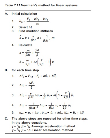
For linear systems as the ones discussed in the chapter there
is no iteration needed. Newmark’s method for linear systems is given in Table
7.11. It is proved that Newmark’s method is stable if
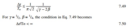
The above proves that the average acceleration method is
stable for any ∆t, no
matter how large; however, it is accurate only if ∆t is small
enough. For the linear acceleration method γ
= 1/2, β = 1/6 and that is stable if
To get an accurate estimate a shorter time step must be used:
The program for Newark’s method’s given in below. Example 7.4
is solved using Newark’s method (γ = 1/2, β = 1/6) - linear acceleration
method - and we get displacement, velocity and acceleration time response as
shown in Fig 7.10.
Program 7.6: MATLAB program for Nemark’s method
for linear systems
%***********************************************************
%
NEWMARK’S METHOD FOR AVERAGE OR LINEAR
ACCELERATION METHODS
%BETA=0.25
.... AVERAGE ACCELERATION METHOD
%BETA = 0.167 .... LINEAR
ACCELERATION METHOD
%*********************************************************** ma=110000;
k=10075582;
wn=sqrt(k/ma)
gamma=0.5
beta=0.25
r=0.07;
c=2.0*r*sqrt(k*ma)
u(1)=0;
v(1)=0;
tt=3.0;
n=300;
n1=n+1
dt=tt/n;
td=.75;
a=ma/(beta*dt)+gamma*c/beta
b=ma/(2.0*beta)+dt*c*(gamma/(2.0*beta)-1) jk=td/dt;
%***********************************************************
% THIS IS WHERE LOAD IS DEFINED
%*********************************************************** for m=1:n1
p(m)=0.0; end jk1=jk+1 for
n=1:jk1 t=(n-1)*dt
p(n)=450000*(1-t/td)*exp(-2.0*t/td)
end
an(1)=(p(1)-c*v(1)-k*u(1))/ma
kh=k+ma/(beta*dt*dt)+gamma*c/(beta*dt) for i=1:n1
s(i)=(i-1)*dt end
for i=2:n1
ww=p(i)-p(i-1)+a*v(i-1)+b*an(i-1) xx=ww/kh
zz=xx/(beta*dt*dt)-v(i-1)/(beta*dt)-an(i-1)/(2.0*beta)
yy=(gamma*xx/(beta*dt)-gamma*v(i-1)/beta+dt*(1-gamma/(2.0*beta))*an(i-1))
v(i)=v(i-1)+yy an(i)=an(i-1)+zz
vv=dt*v(i-1)+dt*dt*(3.0*an(i-1)+zz)/6.0
u(i)=u(i-1)+vv
end figure(1);
plot(s,u,’K’);
xlabel(‘
time (t) in seconds’)
ylabel(‘ Response displacement u in m’) title(‘ dynamic
response’)
figure(2);
plot(s,v,’K’);
xlabel(‘
time (t) in seconds’)
ylabel(‘ Response velocity v in m/sec’) title(‘ dynamic
response’)
figure(3);
plot(s,an,’K’);
xlabel(‘
time (t) in seconds’)
ylabel(‘ Response acceleration a in m/sec’) title(‘ dynamic
response’)
figure(4);
plot(s,p,’K’)
xlabel(‘ time (t) in seconds’)
ylabel(‘ force in Newtons’) title(‘ Excitation Force’)
7.3.8 Conditionally
stable method
Wilson-θ method
A method developed by E L Wilson
is a modification of the conditionally stable linear acceleration method that
makes it unconditionally stable. This is based on the assumption that
acceleration varies linearly over an extended time step δt = θ∆t as shown in Fig. 7.12. The accuracy and stability
properties of the method depend on the value θ which is always greater than 1.
The numerical procedure is derived in a similar line of linear
acceleration methods. Everything described in this chapter will be useful to a
multiple-degrees-of-freedom (MDOF) non-linear system with non-proportional
damping. The incremental velocity and incremental acceleration can be given as
and the incremental velocity and displacement are determined
from Eq. 7.52a, 7.52b. For the MDOF system δui is determined using a
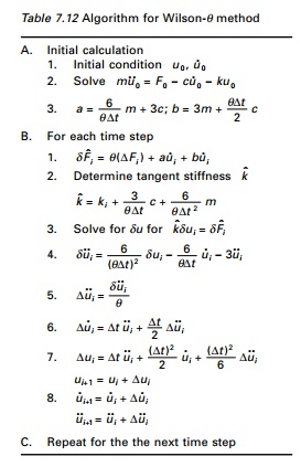
tangent stiffness matrix and an iterative procedure. Table 7.12 gives the
algorithm for the Wilson-θ method.
As discussed earlier, the value
of θ governs the stability characteristics
of the Wilson-θ method.
If θ = 1 this method is the linear
acceleration method, which is stable for ∆t< 0.551 Tn when Tn
is the shortest natural period of time. If θ ≥ 1.37 the
Wilson-θ method
is unconditionally stable, making it suitable for direct solution of

It is proved by Wilson that θ = 1.42 gives optimal accuracy.
The computer program in MATLAB
for Wilson-θ method
for Example 7.4 is given below and we get the displacement. The velocity and
acceleration response are the same as Fig. 7.10.
Program 7.7: MATLAB program for
dynamic response by Wilson-θ Method
% Wilson theta method %********************** ma=110000;
k=10075582;
wn=sqrt(k/ma)
theta=1.42
r=0.07;
c=2.0*r*sqrt(k*ma)
u(1)=0;
v(1)=0;
tt=3.0;
n=300;
n1=n+1
dt=tt/n;
td=.75;
jk=td/dt; for m=1:n1
p(m)=0.0;
end;
jk1=jk+1; for n=1:jk1;
t=(n-1)*dt;
p(n)=450000*(1-t/td)*exp(-2.0*t/td);
end; an(1)=(p(1)-c*v(1)-k*u(1))/ma;
kh=k+3.0*c/(theta*dt)+6.0*ma/(theta*dt)^2;
a=6.0*ma/(theta*dt)+3.0*c;
b=3.0*ma+theta*dt*c/2.0; for
i=1:n1;
s(i)=(i-1)*dt; end;
for i=2:n1;
ww=(p(i)-p(i-1))*theta+a*v(i-1)+b*an(i-1); xx=ww/kh;
zz=(6.0*xx/((theta*dt)^2)-6.0*v(i-1)/(theta*dt)-3.0*an(i-1))/theta;
yy=dt*an(i-1)+dt*zz/2.0;
v(i)=v(i-1)+yy; an(i)=an(i-1)+zz;
vv=dt*v(i-1)+dt*dt*(3.0*an(i-1)+zz)/6.0;
u(i)=u(i-1)+vv;
end;
figure(1);
plot(s,u);
xlabel(‘
time (t) in seconds’)
ylabel(‘ Response displacement u in m’) title(‘ dynamic
response’)
figure(2);
plot(s,v);
xlabel(‘
time (t) in seconds’)
ylabel(‘ Response velocity v in m/sec’) title(‘ dynamic
response’)
figure(3);
plot(s,an);
xlabel(‘
time (t) in seconds’)
ylabel(‘ Response acceleration a in m/sec’) title(‘ dynamic
response’)
figure(4);
plot(s,p)
xlabel(‘ time (t) in seconds’)
ylabel(‘ force in Newtons’) title(‘ Excitation Force’)