Chapter: Civil : Structural dynamics of earthquake engineering
Free vibration of single-degree-of-freedom systems(under-damped)
Free
vibration of single-degree-of-freedom systems (under-damped) in relation to
structural dynamics during earthquakes
Abstract: In this page, the governing
equations of motion are formulated for free vibration of
single-degree-of-freedom (SDOF) (under-damped) systems. Motion characteristics
are studied for under-damped, critically damped and over-damped systems.
Vibration characteristics of an under-damped system are illustrated. Hysteresis
damping and Coulomb damping are also discussed. Programs in MATLAB and in
MATHEMATICA are listed for the vibration of various under-damped SDOF systems.
Key words: viscous damping, logarithmic
decrement, critical damping, hysteresis damping, Coulomb damping.
Introduction
It was seen in the preceding
chapter that a simple oscillator under idealized conditions without damping
will oscillate indefinitely with a constant amplitude at its natural frequency.
In practice, it is not possible to have an oscillator that vibrates
indefinitely. In any practical structure frictional or damping forces will
always be present in the mechanical energy of the system, whether potential or
kinetic energy is transformed to heat energy. In order to account for these
forces, we have to make certain assumptions about these forces based on
experience.
Damping free vibrations
The oscillatory motions
considered so far have been for ideal systems, i.e. systems that oscillate
indefinitely under the action of linear restoring force. In real systems,
dissipative forces, such as friction, are present and retard the motion.
Consequently, the mechanical energy of the system diminishes in time, and the
motion is said to be damped.
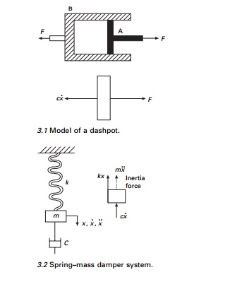
One common type of retarding force is proportional to the
speed and acts in the direction opposite to the motion. The damping caused by
fluid friction is called viscous damping. The presence of this damping
is always modelled by a dashpot, which consists of a piston A moving in a
cylinder B as shown in Fig. 3.1. The frictional force is proportional to velocity
and is denoted by cx˙ and the constant c is called
the coefficient of viscous damping.
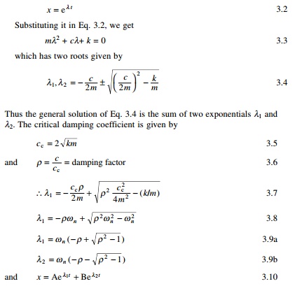
Consider the damped free vibration of a springÐmass damper
system shown in Fig. 3.2. Using D├ĢAlembert├Ģs principle, a dynamic problem can
be converted to a static problem by considering inertia force.
Mx+cx+kx = 0
- - - - -3.1
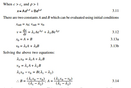
Equation 3.1 is a linear, second order, homogeneous
differential equation. It has the solution of the form
There are three special cases of damping that can be
distinguished with respect to the critical damping coefficient.
Over-damped system
When c > cc and Žü > 1
x = A e╬╗ 1t + Be╬╗ 2t ŌĆ”. 3.11
There are two constants A and B which can be
evaluated using initial conditions
xt=0 = x0;
vt=0 = v0.
As t increases x decreases. This motion is
non-vibratory or a periodic as shown in Fig. 3.3.
Critically damped system
When c = cc and Žü = 1
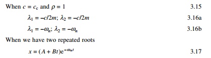
This motion is also non-vibratory
but it is of special interest because x decreases at the fastest
possible rate without oscillation of the mass and is shown in Fig. 3.3.
Under-damped system
When c < cc and Žü < 1. The roots shown in Eq.
3.7 are complex.
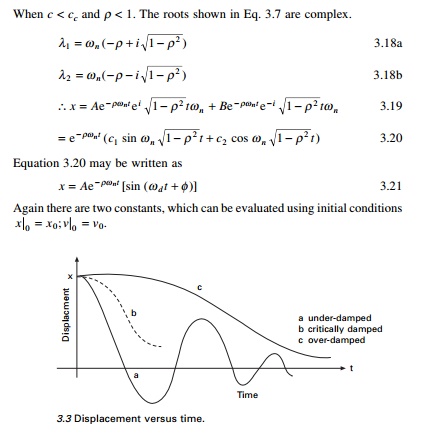
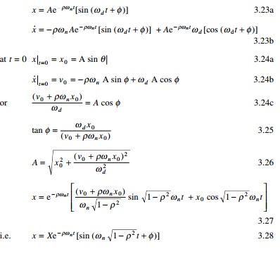
Again there are two constants, which can be evaluated using
initial conditions x 0 = x 0; v 0
= v0.
The constant Žēd is defined as the damped
natural frequency of the system, which is expressed as
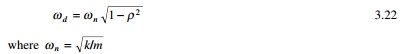
is the natural frequency of the undamped vibration.
Logarithmic decrement
A convenient way to determine the amount of damping present in
a system is to measure the rate of decay of free oscillations. The larger the
damping the greater will be the decay. Consider the damped vibration expressed
by the general equation:

which is shown graphically in Fig. 3.4.
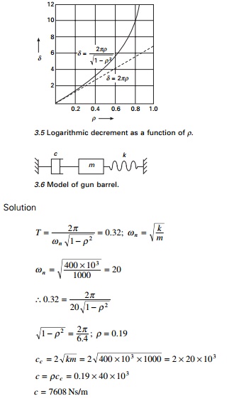
We introduce a term called logarithmic decrement
defined as
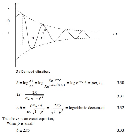
Figure 3.5 shows a plot of the exact and approximate values of
╬┤ as function of Žü.
From Eq. 3.31 it is seen that the period of the damped
vibration Žäd is
constant even though the amplitude decreases

The period of damped vibration is
always larger than the period of the same system without damping.
Example 3.1
A diesel engine generator of mass 1000 kg is mounted on
springs with total stiffness 400kN/m. If the period of oscillation is 0.32s.
determine the damping coefficient c and damping factor Žü.
Given m
= 1000 kg; k = 400 ├- 103
N/m; T = 0.32.
Example
3.2
A gun barrel (Fig. 3.6) weighing 5395.5N has a recoil spring
of stiffness 300 000 N/m. If the gun barrel recoils 1.2 m on firing, determine
(a) the
initial recoil velocity of the barrel;
(b) the
critical damping coefficient of dash pot which is engaged at the end of recoil
stage;
(c) the time
required for the barrel to return to a position 50 mm from its initial
position.
Solution
Weight of gun barrel = 5395.5 N, m = 550 kg, k =
300 000 N/m Kinetic energy = potential energy in the spring
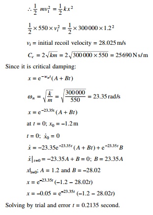
Solving by trial and error t = 0.2135 second.
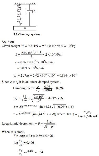
Example 3.3
A vibrating system shown in Fig. 3.7 consists of weight W
= 9.81kN, a spring stiffness 20 kN/cm and a dashpot with coefficient
0.071kN/cm/s., Find (a) damping factor, (b) logarithmic decrement and (c) ratio
of any two consecutive amplitudes.
Example 3.4
A free vibration test is carried out on an empty elevated
water tank shown in Fig. 3.8. A cable attached to the tank applies a lateral
force 144 kN and pulls
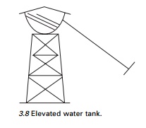
the tank by 0.050 m. Suddenly the
cable is cut and the resulting vibration is recorded. At the end of five
complete cycles, the time is 2 seconds and the amplitude is 0.035m. Compute (a)
stiffness, (b) damping factor, (c) undamped natural frequency, (d) weight of
the tank, (e) damping coefficient and (f) number of cycles when the amplitude
becomes 0.005 m.
Solution
Horizontal
force = F = 144 kN = 144 000 N
Displacement
= u = 0.05 m
(a)
Stiffness = K = F/u =144 000/0.05 =
2 880 000 N/m Time taken for 5 cycles = 2 seconds

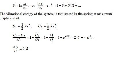
Example 3.5
For small damping, show that the
logarithmic decrement is expressed in terms of vibrational energy U and
the energy dissipated per cycle.
Solution
Hysteresis damping
Real structures and machines do
not exhibit the highly idealized form of viscous damping considered in previous
sections. When materials are cyclically stressed, energy is dissipated within
the material itself due to primarily to internal friction caused by the
slipping and sliding of particles at internal planes during deformations. Such
internal damping is generally referred to as hysteresis damping or structural
damping. This form of damping results in a phase lag between the damping
force and deformation as illustrated in Fig. 3.9. This curve is generally
referred to as a hysteresis loop. The area enclosed within the loop
represents the energy loss or dissipated energy per loading cycle.
If ŌłåU
represents the energy loss per cycle as illustrated in Fig. 3.9 then the energy
loss can be written as
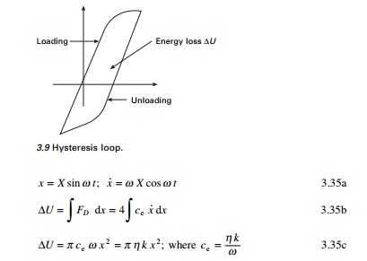
Based on experiments conducted on the internal damping it can
be proved that the energy dissipated per cycle is independent of frequency and
proportional to the square of the amplitude of vibration. Thus, the energy loss
per cycle may be expressed as
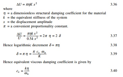
Therefore, for a structure
considered to exhibit hysteretic or structural damping characteristics, the
coefficient ╬Ę can be
determined by measuring successive amplitudes of the oscillation and then
applying Eq. 3.38. Then the structure can be analysed as an equivalent
viscously damped system by calculating the equivalent viscous damping
coefficient calculated from Eq. 3.40.
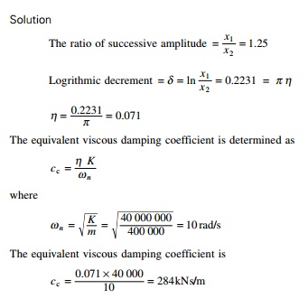
Example 3.6
The main span of a bridge structure is considered as a
single-degree-of-freedom (SDOF) system for calculation of its fundamental
frequency. From preliminary vibration tests, the effective mass of the
structure was determined to be 400 000 kN and the effective stiffness to be 40
000 kN/m. The ratio of successive displacement amplitude from a free vibration
trace was measured to be 1.25. Calculate the values of the structural damping
coefficient and the equivalent viscous damping coefficient.
Coulomb damping
In most of the structures, damping occurs when relative motion
takes place at interfaces or joints between adjacent members. This form of
damping is referred to as Coulomb damping or dry-friction damping.
The friction forces developed are independent of vibration amplitude and
frequency. These forces are acting in the opposite direction of motion of the
mass and the magnitude is essentially constant.
Frictional damping force is given by
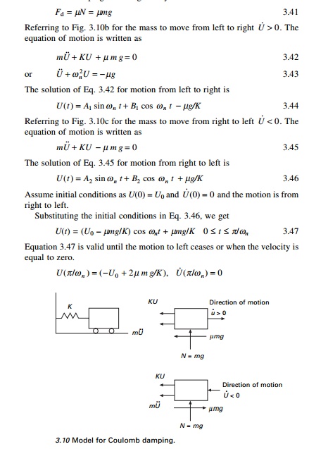
and the motion is from left to right.
Solving for constants in Eq. 3.44 using the conditions at t
= ŽĆ /Žē n
, we get the solution for the displacement as
U(t) = -(U0
- 3┬Ąmg/K) cos Žēnt - ┬Ąmg/K ,,, ,, , ,, 3.48
Substituting when t = 2ŽĆ/Žēn we get
U (2ŽĆ /Žē n ) = (U 0 Ōł' 4 ┬Ą m g/K ), U (2ŽĆ /Žē n ) = 0 --------- - - -3.49
Figure 3.11 shows the free vibration of a system
with Coulomb damping. It is seen that the amplitude decreases by 4Fd/K after
every cycle and the amplitudes decay linearly with time.
Example 3.7
For the system shown in Fig. 3.10W = 1kN; K =
70kN/m; coefficient of friction ’éĄ = 0.15 and the initial conditions are initial
displacement is 0.15m with zero initial velocity. Determine the vibration
displacement amplitude after four cycles and number of cycles of motion
completed before the mass comes to rest.
Solution
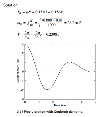
After four cycles displacement amplitude = 150 - 4 ├- 8.57 = 115.72mm
Motion will cease when the
amplitude of the nth cycle such that KUn Ōēż Fd or Un Ōēż 2.14228mm.
150 ├É n ├- 8.57 Ōēż 2.1428 n >17.25 cycles
This indicates that motion will terminate after 17.25 cycles.
Numerical method to
find response due to initial conditions only
The dynamic equation of equilibrium for free
vibration of damped system can be written as
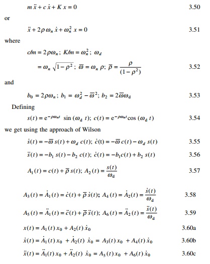
Equation 3.60 gives the relationship between
displacement, velocity and acceleration with time.
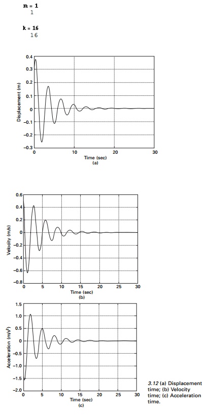
Program 3.1: MATLAB
program for free vibration of under-damped (SDOF) systems
clc close all
%****************************************************
% give mass of the system
m=2;
%give stiffness of the system
k=8;
wn=sqrt(k/m);
%give damping coefficient c1=1;
%give initial conditions -
displacement and velocity u(1)=.3;
udot(1)=.5; uddot(1)=(-c1*udot(1)-k*u(1))/m;
%****************************************************
cc=2*sqrt(k*m);
rho=c1/cc;
wd=wn*sqrt(1-rho^2);
wba=rho*wn;
rhoba=rho/sqrt(1-rho^2);
b0=2.0*rho*wn;
b1=wd^2-wba^2;
b2=2.0*wba*wd;
dt=0.02;
t(1)=0;
for i=2:1500
t(i)=(i-1)*dt;
s=exp(-rho*wn*t(i))*sin(wd*t(i));
c=exp(-rho*wn*t(i))*cos(wd*t(i)); sdot=-wba*s+wd*c; cdot=-wba*c-wd*s;
sddot=-b1*s-b2*c; cddot=-b1*c+b2*s; a1=c+rhoba*s;
a2=s/wd;
a3=cdot+rhoba*sdot;
a4=sdot/wd;
a5=cddot+rhoba*sddot;
a6=sddot/wd;
u(i)=a1*u(1)+a2*udot(1);
udot(i)=a3*u(1)+a4*udot(1);
uddot(i)=a5*u(1)+a6*udot(1); end
figure(1);
plot(t,u,├'k├Ģ); xlabel(├' time├Ģ);
ylabel(├' displacement ├Ģ); title(├'
displacement - time├Ģ); figure(2);
plot(t,udot,├'k├Ģ); xlabel(├'
time├Ģ); ylabel(├' velocity├Ģ); title(├' velocity - time├Ģ); figure(3);
plot(t,uddot,├'k├Ģ); xlabel(├' time├Ģ); ylabel(├' acceleration├Ģ);
title(├' acceleration- time├Ģ);
The displacement time, velocity time and
accelertion time curves are shown in Fig. 3.12.
Program 3.2: MATHEMATICA program for free
vibration of damped SDOF systems
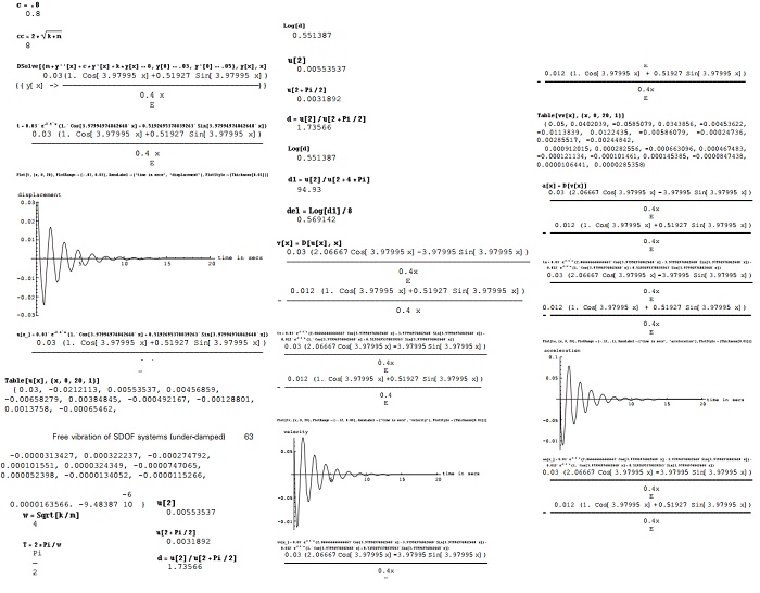
{0.05, 0.0402039, -0.0585079, 0.0343856,
-0.00453622, -0.0113839, 0.0122435, -0.00586079, -0.00024736, 0.00285517,
-0.00244842,
0.000912015, 0.000282556, -0.000663096, 0.000467483,
-0.000121134, -0.000101461, 0.000145385, -0.0000847438, 0.0000106441,
0.0000285358}
Summary
Real structures dissipate energy while undergoing
vibratory motion. The common method is to assume that dissipated energy is
proportional to damping forces. Damping forces are proportional to velocity
acting in the opposite direction of motion. The analytical expression for the
solution of the governing differential equation depends on the magnitude of the
damping ratio. Three cases are possible: (i) under-damped system, (ii)
critically damped system, and (iii) over-damped system. A practical method of
determining the damping present in a system is to evaluate experimentally the
logarithmic decrement which is defined as the natural logarithm of the ratio of
two consecutive peaks in free vibration. The damping ratio in buildings and
bridges is usually less that 20% of critical damping. For such systems the
damped frequency is equal to the undamped natural frequency.
Related Topics