Two-degrees-of-freedom linear system response of structures

Two-degrees-of-freedom linear system response of structures

Abstract: This chapter deals with the free and forced vibration of two-degrees-of-freedom systems. Coordinate coupling is illustrated by means of an example. The concept behind the vibration absorber is given.

Key words: beat, dynamic coupling, static coupling, vibration absorber, positive definite.

Overview

In many textbooks the concepts presented in the previous chapters are extended from a single-degree-of-freedom (SDOF) system to a multiple-degrees-of-freedom (MDOF) system without first presenting the solutions for the two-degrees-of-freedom system. Such an approach does not allow readers to gradually learn the methodology and also means many important structural engineering concepts are not presented. Therefore, this page is devoted to the two-degrees-of-freedom system.

When a system requires two coordinates to describe its motion, it is said to have two degrees of freedom. A two-degrees-of-freedom system will have two natural frequencies when free vibration takes place at one of these natural frequencies, a definite relationship exists between the amplitude of the two coordinates and the configuration is referred to as normal mode. The two-degrees-of-freedom system will then have two natural modes of vibrations corresponding to the two natural frequencies. For a linear system, free vibration initiated under any condition will in general be the two normal modes of vibration.

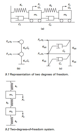
Free vibration of a two-degrees-of-freedom system will be taken first, and then its forced vibration characteristics dealt with. There are many ways that a two-degrees-of-freedom system can be represented, three of which are shown in Fig. 9.1.

Free vibration of undamped two-degrees-of-freedom system

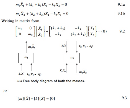
The system shown in Fig. 9.2 has two masses m1 and m2 connected by springs of stiffness k1, and k2. It is a two-degrees-of-freedom system and the configura-tion is fully described by two displacements x1 and x2 as shown in Fig. 9.2.

Writing the dynamic equations of equilibrium, considering the free body diagrams shown in Fig. 9.3, we get

[ m ]{ X } + [ k ]{ X} = {0}                    9.3

One can identify [m] as mass matrix and [k] as stiffness matrix. {m} and [k] are symmetric and positive definite. Mass matrix is uncoupled and stiffness matrix is coupled and hence it is known as dynamically uncoupled and statically coupled system.

Try a solution

X1 = A1 sin (ωnt + Ï†); X2 = A2 sin (ωnt + Ï†)      9.4

Equation 9.6 involves two homogeneous equations. A trivial solution is A1 = A2 = 0. Equation 9.6 is rewritten as

For a non-trivial solution to exist, the determinant of the above matrix should be equal to zero. Simplification yields the characteristic equation as

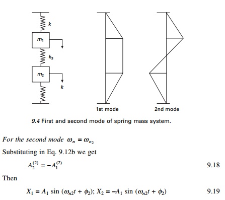
Then the system vibrates in first mode as shown in Fig. 9.4. In the first normal mode, two masses move in phase as shown in Fig. 9.4 and the centre spring is not compressed.

X1 = A1 sin (ωn2t + Ï†2); X2 = â€'A1 sin (ωn2t + Ï†2)         9.19

The second mode is also plotted in Fig. 9.4. In the second normal mode, the masses move in opposition, out of phase with each other. For the second mode there is one node, which is the point other than support at which displacement is zero. For the

mth mode there must be (m â€' 1) nodes.

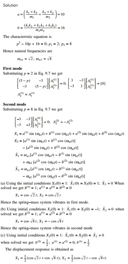
Example 9.1

k = 2; k3 = 3; m1 = m2 = 1 (See Fig. 9.2). Find the natural frequencies. Find

The solution of a coupled differential equation is performed using MATHEMATICA, including response curves. The program in MATHEMATICA is given below.

Program 9.1: MATHEMATICA program to solve coupled differential equation (program not given)

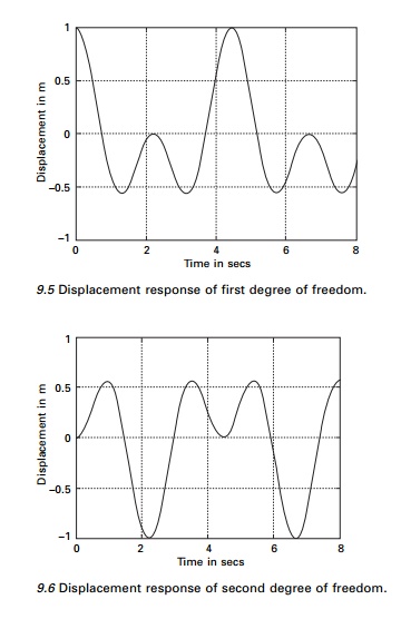
Program 9.2: MATLAB program to solve free vibration of undamped two-degrees-of-freedom system

%two degrees of freedom forced vibration undamped clc;

mass matrix

m=[1 0;0 1];

%stiffness matrix k=[5 -3;-3 5];

%give initial displacements and velocities u=[1 0 0 0];

%calculate flexibility matrix

a=inv(k);

am=a*m;

%find eigen values and eigenvectors [ev,evu]=eig(am);

%calculate frequencies and factors for i=1:2

omega(i)=sqrt(1/evu(i,i));

mew(i)=ev(i,2)/ev(i,1); end

%find b matrix

b=[0 1 0 1;omega(1) 0 omega(2) 0;0 mew(1) 0 mew(2);...

omega(1)*mew(1) 0 omega(2)*mew(2) 0]; a=inv(b)*u’;

for i=1:401 tt(i)=(i-1)*.02; t=tt(i);

bb=[sin(omega(1)*t) cos(omega(1)*t) sin(omega(2)*t) cos(omega(2)*t); o m e g a ( 1 ) * c o s ( o m e g a ( 1 ) * t ) - o m e g a ( 1 ) * s i n ( o m e g a ( 1 ) * t ) omega(2)*cos(omega(2)*t)...

-omega(2)*sin(omega(2)*t); mew(1)*sin(omega(1)*t)mew(1)*cos(omega(1)*t) mew(2)*sin(omega(2)*t)

mew(2)*cos(omega(2)*t);...

mew(1)*omega(1)*cos(omega(1)*t) -mew(1)*omega(1)*sin(omega(1)*t)...

mew(2)*omega(2)*cos(omega(2)*t) -omega(2)*mew(2)*sin(omega(2)*t)] c=bb*a

u(i)=c(1);

v(i)=c(3); end

figure(1)

plot(tt,u)

xlabel(‘ time in secs’) ylabel(‘ displacement in m’)

title(‘ response first degree of freedom’) figure(2)

plot(tt,v)

xlabel(‘ time in secs’) ylabel(‘ displacement in m’)

title(‘ response second degree of freedom’) igure(2)

Program 9.3: MATLAB program to solve coupled differential equations

MATLAB has several functions or solvers, based on the use of Rungeâ€'Kutta methods that can be used for the solution of a system of first order ordinary differential equations. It is to be noted that nth order ordinary differential equations are converted to n first order ordinary differential equations before using the MATLAB functions. The MATLAB function ode23 implements a combination of second and third order Rungeâ€'Kutta methods while the function ode45 is based on a combination of fourth and fifth order Rungeâ€'Kutta methods. To solve a system of first order differential equation yË™ = f ( t , y) using MATLAB function ode23, the following command can be used

[t,y]=ode23[‘dfunc’,tspan,y0]

where ‘dfunc’ is the name of the function m-file whose input must be t and y and whose output must be a column vector denoting dy/dt on f (t, y). The number of rows in the column vector must be equal to the number of first order equations. The vector ‘tspan’ should contain the initial and final values of the independent variable t, and optimally any intermediate value of ‘t’ at which the solution is desired. The vector y0 should contain the initial values of y(t). The function ‘m-file’ should have two input arguments t and y. A similar procedure can be used with MATLAB functions ode45.

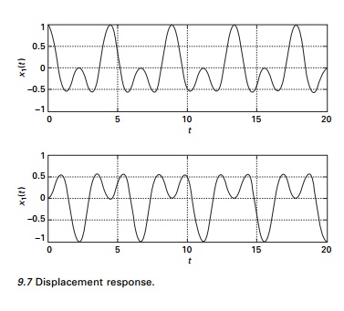
Assume y1, y3 represent the displacements x1 and x2 and the two second order equations can be converted to four first order equations as

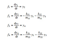
The problem discussed in MATHEMATICA is solved using MATLAB. Figure 9.7 shows the displacement response.

%Matlab program for solving coupled differential equation using RK method tspan=[0:.01:20];

%Initial displacements and velocities y0=[1.0;0.0;0.0;0.0];

%Use RK method of order 4 and 5 combined [t,y]=ode45(‘dfunc1’,tspan,y0);

subplot(211)

plot(t,y(:,1)); xlabel(‘t’); ylabel(‘x1(t)’);

title(‘ x1(t) vs t’); subplot(212) plot(t,y(:,3)); xlabel(‘t’); ylabel(‘x2(t)’); title(‘x2(t) vs t’);

function f=dfunc1(t,y)

% four first order equations are given by f f=zeros(4,1);

%mass matrix m=[1,0;0,1]; %stiffness matrix k=[5 -3;-3 5];

%four first order equations f(1)=y(2);

f(2)=-k(1,1)*y(1)/m(1,1)-k(1,2)*y(3)/m(1,1); f(3)=y(4); f(4)=-k(2,1)*y(1)/m(2,2)-k(2,2)*y(3)/m(2,2);

Example 9.2

Assume k1 = k2 = 1.7; k3 = 0.3. Investigate the beating phenomenon assuming the initial conditions as X1(0) = 1: X1 (0) = X2(0) = = 0 .

The beating phenomenon is shown in Fig. 9.8 and the curves are obtained using the MATLAB package. The resulting motion is a rapid oscillation with

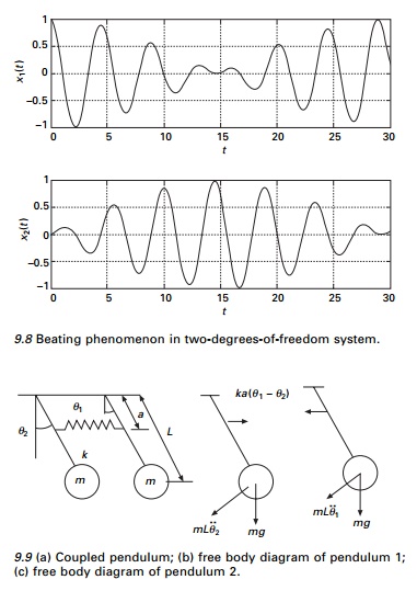
a slowly varying period and is referred as beat. Sometimes the two sinusoids add to each other, and all other times they cancel each other out, resulting in a beating phenomenon. The beating phenomenon often manifests itself in mechanical equipment with the emitted sound having a similar cyclically varying magnitude.

Example 9.3

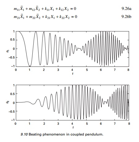
In Fig. 9.9 two pendulums are coupled by means of a weak spring k, which is unconstrained when two pendulum rods are in the vertical position. Determine the normal modes of vibration.

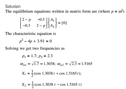
Solution

Assuming anticlockwise angular displacement to be positive and taking moments about the point of suspension, we obtain the following equations of motion for small oscillation.

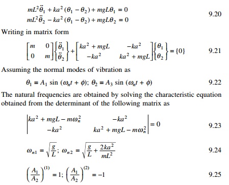
Thus in the first mode the two pendulums move in phase and the spring remains unstretched. In the second mode, the two pendulums are out of phase and the coupling is actively involved with a node at its midpoint. Consequently the natural frequency is higher. In the coupled pendulum assume m1 = m1 = 0.1; k = 5; a = 0.4 m; L = 1m. We get the beating phenomenon as shown in Fig. 9.10. A MATLAB program using ode45 can be used to find the response of the pendulums.

Coordinate coupling

The differential equations of motion for the two-degrees-of-freedom system are in general coupled. In that both coordinates appear in each equation. In the most general case, the two equations of the undamped system have the following form:

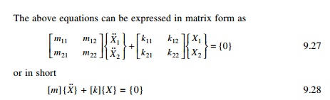
In the above equations, the mass and stiffness matrices are non-diagonal. Hence mass or dynamic coupling and stiffness or static coupling exist.

It is also possible to find the coordinate system which has neither form of coupling. The two equations are then decoupled and each equation may be solved independently of the other. For example {X} is written in terms of some other coordinate as

{Y} coordinates are called principal coordinates or normal coordinates. Although it is possible to decouple the equations of motion for an undamped

system, this is not the case for the damped system. The following system of equations show uncoupled mass and stiffness matrices but coupled damping matrix.

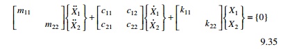
If in Eq. 9.35 c12 = c21 = 0 then damping is said to be proportional damping. The damping matrix is also uncoupled when we assume damping is proportional to stiffness and mass matrices.

Example 9.4

Figure 9.11 shows a rigid bar of an automobile with its centre of mass not coinciding with its geometric centre . L1 â‰  L2 and supported by two springs of stiffness k1, k2. This represents a two-degrees-of-freedom system since two coordinates are necessary to describe its motion. The choice of coordinates will define the type of coupling.

Solution

1.     Choose coordinates X and Î¸ as the displacement at centre of mass and rotation of rigid bar (see Fig. 9.11b). The free body diagram is shown in Fig. 9.12.

Writing the equations of dynamic equilibrium we get

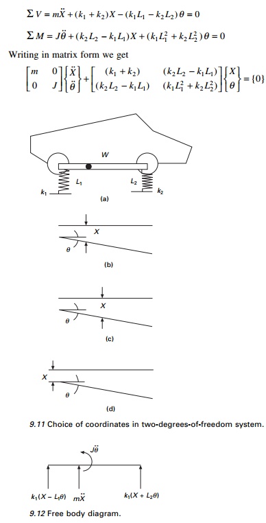
The above equations show mass or dynamic uncoupling and static or stiffness coupling. If k1L1 = k2L2 we obtain uncoupled X and Î¸ vibration. Then stiffness matrix is also uncoupled.

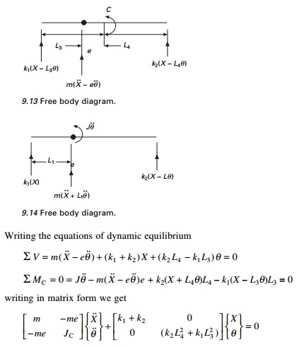
2.Choose coordinates X and Î¸ as displacements at the centre of gravity C of the bar as shown in Fig. 9.11c and rotation of the bar. Assume C is selected such that k1L3 = k2L4. The free body diagram is shown in Fig. 9.13.

In the above equations, mass matrix is coupled (dynamic coupling) and stiffness matrix is uncoupled (static uncoupling).

3.     Choose the coordinates X and Î¸ such that X is the displacement at the left support and Î¸ is the rotation of the rigid bar as shown in Fig. 9.11d. The free body diagram is shown in Fig. 9.14.

Writing the dynamic equations of equilibrium, we get

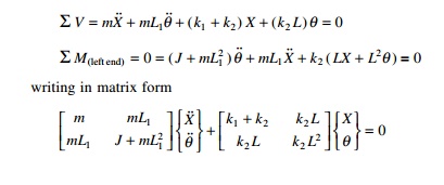
In the above equation, mass and stiffness matrices are coupled and hence there exists both dynamic and static coupling. This example shows the choice of coordinates will define the types of coupling which can immediately be determined for the mass and stiffness matrices.

Simple system: two storey shear building

1.   Influence coefficient method

The influence coefficients associated with stiffness and mass matrices are respectively known as stiffness and inertia influence coefficients. The inverse of stiffness matrix is the flexibility matrix. kij is the stiffness influence coefficient defined as the force developed at ‘i’ due to unit force applied at ‘j’. We first formulate the equation of motion for the simplest possible two-degrees-of-freedom system, a highly idealized two storey frame. In this idealization, the beams and floor systems are rigid (infinitely stiff) in flexure. Axial deformations in the beams and columns and the effect of axial force on stiffness of the columns are neglected. Even though it is unrealistic nevertheless we can illustrate how equations of motion for an MDOF system are developed. Consider a two storey frame shown in Fig. 9.15.

The equation of motion may be written as

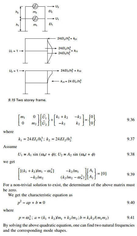
Example 9.5

In the above two storey shear frame problem

m1 = m; m2 = 0.5m; k1 = k2 = k

Find the natural frequencies and mode shapes.

p2 â€' (4 k/m)p + 2(k/m) = 0

Solving

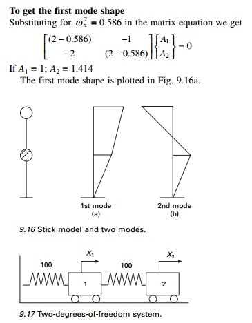
To get the first mode shape

Substituting for Ï‰ n2  = 0.586 in the matrix equation we get

To get the second mode shape

Substituting for Ï‰ n2  = 3.414 in the matrix equation we get

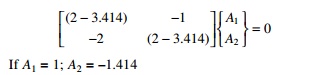
The second mode shape is plotted in Fig. 9.16b.

Example 9.6

Solve the two-degrees-of-freedom system shown in Fig. 9.17 by Laplace transform. Obtain the response given initial conditions initial displacements corresponding to two degrees of freedom are 3 and 5 respectively and initial velocities corresponding to two degrees of freedom are 1 and 4 respectively.

Solution

The equations of motion can be written as

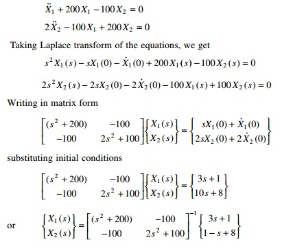
Taking inverse Laplace transform we will get X1(t), X2(t). The program in MATHEMATICA is given below and the response curves are shown for both the displacements.

Forced vibration of two-degrees-of-freedom undamped system

It is required to study the steady state response of the system shown in Fig. 9.21 when the mass m1 is excited by the force F1 = F10 cos(ω t) and also to plot the frequency response curve.

Dynamic equations of equilibrium can be written as

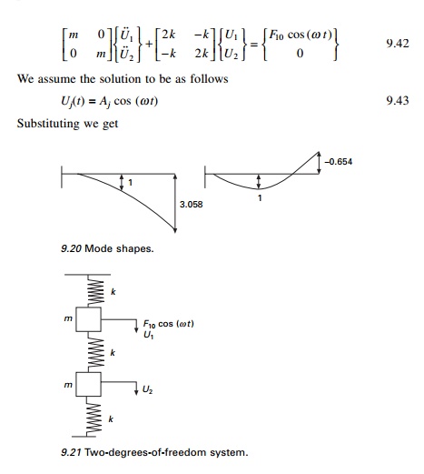
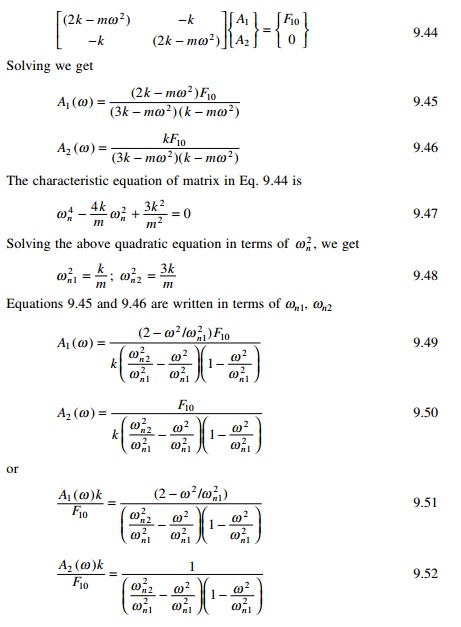
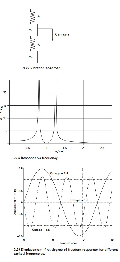
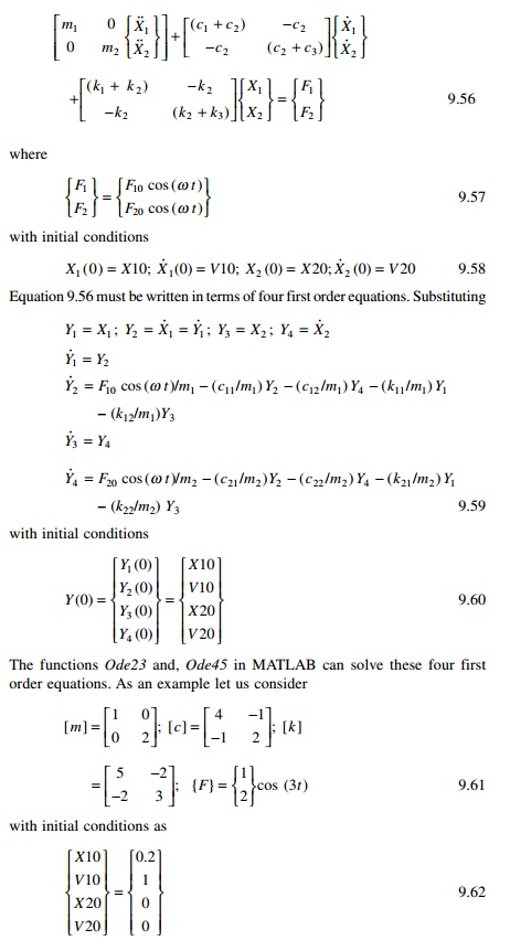
The responses A1 and A2 are shown on page 296 respectively in terms of dimensionless parameter Ï‰/ω1. In the dimensionless parameter Ï‰/ω1 Ï‰1 is selected arbitrarily. It can be seen that amplitudes of U1 and U2 become infinity when Ï‰ 2 = Ï‰ n21 or Ï‰ 2 = Ï‰ n22 . These are the resonance conditions for the system, one at Ï‰n1 and the other at Ï‰n2. At all other values of Ï‰, the amplitudes of vibration are finite. It can be noted from the figure on previews page that there is a particular value of frequency Ï‰ at which the vibration of first mass m to which force F1 is applied is reduced to zero. This concept is made use of in vibration absorbers.

Vibration absorber

A spring mass system k2, m2 tuned to the frequency of the exciting force such that Ï‰2 = k2/m2 will act as a vibration absorber and reduce the motion of the main mass m1 to zero (see Fig. 9.22).

Assuming the motion to be harmonic, the equation for amplitude can be shown equal to that given by Eq. 9.54 by substituting for fundamental frequencies given by Eq. 9.53.

Assume m1 = 1; m2 = 0.2; k1 = 1; k2 = 0.2; Ï‰112 = k1/m1 = 1; Ï‰ 222 = k2/m2 = 1. Figure 9.23 shows a plot of Eq. 9.54. If Ï‰ = Ï‰22 the amplitude A1 = 0 but the absorber mass undergoes an amplitude equal to

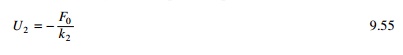
since the force acting on m2 is â€'F0. The absorber system k2, m2 exerts a force equal and opposite to the disturbing force. Thus the size of k2, m2 depends on the allowable value of U2.

Figures 9.24 and 9.25 show the response of both degrees of freedom by varying the excited frequency. It is seen that when the excited frequency = 1rad/s the displacement corresponding to the first degree of freedom is zero.

9.24 Displacement (first degree of freedom response) for different excited frequencies.

Forced response of a two-degrees-of-freedom under-damped system

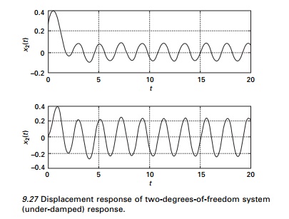
Consider a two-degrees-of-freedom under-damped system as shown in Fig. 9.26. The equations of motion can be written in matrix form as shown in Eq.

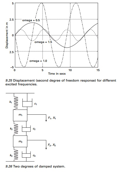
Figure 9.27 shows the displacement response for this two-degrees-of-freedom system.

The program in MATLAB is given below.

Program 9.6: MATLAB program for displacement response of two-degrees-of-freedom under-damped system for forced vibration

%FORCED RESPONSE OF TWO DEGREE OF FREEDOM UNDER DAMPED SYSTEM

tspan=[0:.01:20];

y0=[0.2;1.0;0.0;0.0]; [t,y]=ode45(‘dfunc’,tspan,y0); subplot(211)

plot(t,y(:,1)); xlabel(‘t’); ylabel(‘x1(t)’); title(‘ x1(t) vs t’); subplot(212) plot(t,y(:,3)); xlabel(‘t’); ylabel(‘x2(t)’); title(‘x2(t) vs t’);

function f=dfunc(t,y) f=zeros(4,1);

m=[1 0;0 2]; c=[4 -1;-1 2]; k=[5 -2;-2 3]; force=[1;2]; om=3.0; f(1)=y(2);

f(2)=force(1)*cos(om*t)-c(1,1)*y(2)/m(1,1)-c(1,2)*y(4)/m(1,1)...

-k(1,1)*y(1)/m(1,1)-k(1,2)*y(3)/m(1,1); f(3)=y(4);

f(4)=force(2)*cos(om*t)-c(2,1)*y(2)/m(2,2)-c(2,2)*y(4)/m(2,2)...

-k(2,1)*y(1)/m(2,2)-k(2,2)*y(3)/m(2,2);

9.14      Summary

In this chapter, response of two-degrees-of-freedom system undamped and under-damped free vibration and forced vibration is discussed. The relevant programs in MATHEMATICA and MATLAB are given. In the next chapter, free vibration of multiple-degrees-of-freedom systems is discussed.