Chapter: Civil : Structural dynamics of earthquake engineering
Elastic design spectrum
Elastic design spectrum
Although the recorded ground
acceleration and response spectra of past earthquakes provide a basis for the
rational design of structures to resist earthquakes, they cannot be used
directly in design, since the response of a given structure to past earthquakes
will invariably be different from its response to a future earthquake. However,
certain similarities exist among earthquakes recorded under similar conditions.
These characteristics have been discussed in previous sections on response
spectra. Earthquake data with common characteristics have been averaged and
ŌĆśsmoothedŌĆÖ to create ŌĆśdesign spectraŌĆÖ.
1NewmarkŌĆōHall ŌĆśbroad-bandedŌĆÖ designs spectrum
This spectrum is normalized to a maximum ground acceleration
of 1.0g. The maximum ground velocity is specified by 1219.2 mm/s and
maximum ground displacement is 914.4 mm. The principal regions (acceleration,
velocity and displacement) of the design spectrum are identified in which the
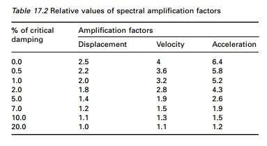
response is approximately a constant, amplified value. Amplification factors
are then applied to the maximum ground motion in these regions to obtain the
desired design spectrum. The procedure is as follows:
1. Plot
the anticipated ground motion polygon on four-way logarithmic paper.
2. Apply
the appropriate amplification factor presented in Table 17.2 with maximum ground motion to construct design
spectrum for specific damping values.
3. Draw
the amplified displacement bound parallel to maximum ground motion
displacement.
4. Draw
the amplified velocity bound parallel to maximum ground velocity.
5. Draw
the amplified acceleration bound parallel to maximum ground acceleration.
6. Below a
period of 0.17 s the amplified acceleration bound approaches the maximum ground
acceleration. Draw a straight line from the amplification acceleration bound at
0.17 s to the maximum ground acceleration line at 0.033 s.
7. Below a
period of 0.033 s the acceleration bound is the same as maximum ground
acceleration.
In general, the spectral
intensities for vertical motion can be taken as approximately two-thirds of
horizontal motion when the fault positions are horizontal. Where fault motions
are expected to involve large vertical components, the spectral intensity,
vertical motion is assumed to be equal to horizontal.
Example 17.6
Construct a NewmarkŌĆōHall design
spectrum for a maximum ground acceleration equal to that of Northridge
earthquake 0.308g and for concrete buildings.
Solution
(a) Determine
maximum ground motion parameters Maximum ground acceleration | u˙˙g (t ) | = 0.308g
Maximum ground velocity
= 1219.2 ├Ś 0.308
| u˙ g
(
t ) |max =
375.5mm/s
Maximum ground displacement = 914.4 ├Ś 0.308
| Ug(t)
|max = 281.63
mm
(b)Determine the amplified response parameters for p =
0.05
From table amplified Spa = 2.6 ├Ś 0.308g
= 0.801g m/s2
Amplified Spv = 1.9 ├Ś 375.5
= 713.45 mm/s
Amplified Spd = sd = 1.4 ├Ś 281.63
= 394.28 mm
(b) Construction
of design spectrum
(i)
Draw the maximum ground motion polygon using | u˙˙g ( t ) |max,
| u˙ g
(t
) | max, | u g (t ) |max .
(ii)Draw the amplified displacement Sd bound
parallel to the maximum ground displacement.
(iii) Draw the
amplified velocity Sv parallel to the maximum ground velocity
line. It intersects displacement bound at T1 = 3.5 s.
(iv) Draw the
amplified acceleration Spa bound to maximum ground
acceleration. It intersects velocity bound at 0.55 = T2.
Extend the amplified acceleration bound downward left to the point
corresponding to T3 = 0.17.
(v) Draw the
amplified acceleration bound linearly from the point corresponding to T3
= 0.17 so that it intersects a line at T4 = 0.033 s with
maximum ground acceleration.
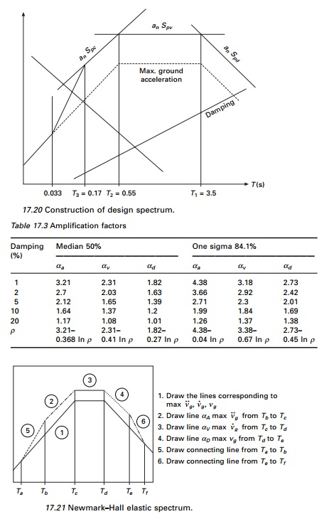
This spectrum is shown in Fig. 17.20.
Researchers have developed
procedures to construct the design spectra. From the ground motion parameters
the recommended values for firm ground are Ta = 1/33; Tb
= 1/8; Te = 10; Tf = 33 s. The
amplification factors for ╬▒a, ╬▒v, ╬▒d for Spa,
Spv, Sd were developed for two different
non-accedence probabilities 50% and 84.1% as given in Table 17.3. NewmarkŌĆōHall
elastic spectrum construction is shown in Fig. 17.21.
Program 17.3: MATLAB
program for drawing NemarkŌĆōHall design spectra
%********************************************************** %
TO DRAW ELASTIC DESIGN NEWMARK-HALL SPECTRA
%**********************************************************
%give ip=1 for 50% mean and ip=2
for 84.1% median ip=1
%**********************************************************
c=[3.21 4.38;2.31 3.38;1.82 2.73];
d=[-.68 -1.04;-.41 -0.67;-.27
-.45]; %**********************************************************
%give damping value rho
%********************************************************** rho=5
%**********************************************************
%**********************************************************
%give peak ground acceln, peak
ground velocity peak ground disp %**********************************************************
pga=981.0;
pgv=121.92;
pgd=91.44;
ca=c(1,ip)+d(1,ip)*log(rho);
cv=c(2,ip)+d(2,ip)*log(rho);
cd=c(3,ip)+d(3,ip)*log(rho); for
k=.00001:.00001:.0001 x=0.01:1:100 t=log(2*pi*k)-log(x) y=exp(t)
loglog(x,y,ŌĆśkŌĆÖ),grid on
hold on
t=log(k*9.81/(2*pi))+log(x) y=exp(t)
loglog(x,y,ŌĆśkŌĆÖ) hold on
end
for k=.0001:.0001:.001
x=0.01:1:100 t=log(2*pi*k)-log(x) y=exp(t) loglog(x,y,ŌĆśkŌĆÖ),grid on hold on
t=log(k*9.81/(2*pi))+log(x)
y=exp(t)
loglog(x,y,ŌĆśkŌĆÖ) hold on
end
for k=.001:.001:.01 x=0.01:1:100
t=log(2*pi*k)-log(x) y=exp(t) loglog(x,y,ŌĆśkŌĆÖ),grid on hold on
t=log(k*9.81/(2*pi))+log(x)
y=exp(t)
loglog(x,y,ŌĆśkŌĆÖ) hold on
end
xlabel(ŌĆś period in secsŌĆÖ)
ylabel(ŌĆś spectral velocity sv in
cm/secŌĆÖ) for k=.01:.01:.1
x=0.01:1:100 t=log(2*pi*k)-log(x) y=exp(t)
loglog(x,y,ŌĆśkŌĆÖ),grid on hold on
t=log(k*9.81/(2*pi))+log(x)
y=exp(t)
loglog(x,y,ŌĆśkŌĆÖ) hold on
end
for k=.1:.1:1 x=0.01:1:100
t=log(2*pi*k)-log(x) y=exp(t) loglog(x,y,ŌĆśkŌĆÖ),grid on hold on
t=log(k*9.81/(2*pi))+log(x)
y=exp(t)
loglog(x,y,ŌĆśkŌĆÖ) hold on
end
for k=1:1:10 x=0.01:1:100
t=log(2*pi*k)-log(x) y=exp(t) loglog(x,y,ŌĆśkŌĆÖ),grid on hold on
t=log(k*9.81/(2*pi))+log(x)
y=exp(t)
loglog(x,y,ŌĆśkŌĆÖ) hold on
end
for k=10:10:100 x=0.01:1:100
t=log(2*pi*k)-log(x) y=exp(t) loglog(x,y,ŌĆśkŌĆÖ),grid on hold on
t=log(k*9.81/(2*pi))+log(x)
y=exp(t)
loglog(x,y,ŌĆśkŌĆÖ) hold on
end
for k=100:100:1000 x=0.01:1:100 t=log(2*pi*k)-log(x) y=exp(t)
loglog(x,y,ŌĆśkŌĆÖ),grid on
hold on
t=log(k*9.81/(2*pi))+log(x) y=exp(t)
loglog(x,y,ŌĆśkŌĆÖ) hold on
end
for k=1000:1000:10000
x=0.01:1:100 t=log(2*pi*k)-log(x) y=exp(t) loglog(x,y,ŌĆśkŌĆÖ),grid on hold on
t=log(k*9.81/(2*pi))+log(x)
y=exp(t)
loglog(x,y,ŌĆśkŌĆÖ) end
axis([0.01 100 0.02 500])
text(0.2,0.02,ŌĆś0.001ŌĆÖ); text(0.6,0.1,ŌĆś0.01ŌĆÖ); text(2,0.3,ŌĆś0.1ŌĆÖ); text(7,1,ŌĆś1ŌĆÖ);
text(20,3,ŌĆś10ŌĆÖ); text(80,10,ŌĆś100ŌĆÖ) text(20,1,ŌĆśSd in cmŌĆÖ) xlabel(ŌĆś period in
secŌĆÖ) ylabel(ŌĆś Sv in cm/secŌĆÖ) text(0.01,200,ŌĆś100ŌĆÖ) text(0.01,20,ŌĆś10ŌĆÖ)
text(0.01,2,ŌĆś1ŌĆÖ) text(0.02,0.4,ŌĆś0.1ŌĆÖ) text(0.07,0.1,ŌĆś0.01ŌĆÖ)
text(.02,0.8,ŌĆśSa/gŌĆÖ) xc(1)=0.01; xc(2)=0.0303; xc(3)=0.125;
xc(4)=cv*pgv*2*pi/(ca*pga);
xc(5)=cd*pgd*2*pi/(cv*pgv);
xc(6)=10;
xc(7)=33.0
xc(8)=100.0;
yc(1)=pga*0.01/(2.0*pi);
yc(2)=pga*0.0303/(2*pi);
yc(3)=ca*pga*0.125/(2*pi);
yc(4)=cv*pgv;
yc(5)=cv*pgv;
yc(6)=cd*pgd*2*pi/10;
yc(7)=pgd*2*pi/33;
yc(8)=pgd*2*pi/100;
line(xc,yc,ŌĆślinewidthŌĆÖ,3,ŌĆścolorŌĆÖ,ŌĆśkŌĆÖ);
title(ŌĆś Newmark- Hall Design Spectrum 50% Median and rho=5%ŌĆÖ)
Related Topics