Earthquake response spectra

Earthquake response spectra

Abstract: In this chapter, earthquake excitation problems are treated as base excitation problems. In many engineering applications, one requires maximum absolute quantities experienced by the structure during the earthquake of interest. In that respect, the response spectrum method is ideally suited to designing structures against earthquake motion. It is shown how the tripartite plot is useful for reading all the spectral quantities for a given period. The construction of a Newmark–Hall design spectrum is illustrated and the distinction is made between design and response spectra. In all the codes, site-specific response spectra are recommended. Finally inelastic design spectra are also discussed.

Key words: accelerograph, response spectrum, spectral quantity, pseudo spectral quantity, ductility, time history.

Introduction

The earthquake response problem is essentially a base excitation problem similar to the one discussed in the earlier chapter for single-degree-of-freedom (SDOF) systems. The equation of motion is written as

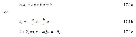
Thus for any arbitrary acceleration of the supports the relative displacement of the mass can be computed using the Duhamel integral as

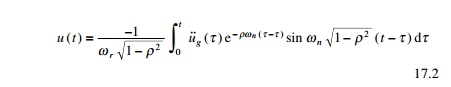
From Eq. 17.2 it is seen that the relative response of the structure is characterized by its natural frequency, damping factor and the nature of base excitation.

Generally we use undamped natural frequency instead of damped frequency and the negative sign is ignored (the sense of response has no significance in earthquake analysis)

v(t) = R(t) is called the earthquake response integral. The relative displacement is important since it is required to calculate base shear.

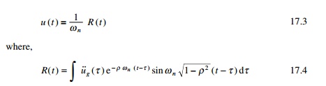
It is noticed that base shear represented in Eq. 17.5 is equivalent to restoring force F_s(t). The exact relative velocity is given by

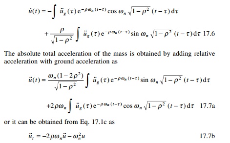
The absolute total acceleration of the mass is obtained by adding relative acceleration with ground acceleration as

The total acceleration has many important applications. It can most easily be measured experimentally during a strong earthquake. When an accelerograph is located in a structure, it records in close approximation the total acceleration at that point. From this we can calculate inertia force

Equations 17.2, 17.6 and 17.7 represent the earthquake time history response for an SDOF system. Once we know base shear V (effective earthquake force), we can design a system.

Earthquake response spectra

It has been seen from earlier chapters that the evaluation of dynamic response (displacement, velocity and acceleration) at every instant of time during an earthquake requires significant computational effort even for relatively simple structural systems. However, for many engineering applications we require maximum absolute quantities experienced by the structure during the earthquake. These are commonly referred to as spectral displacement S_d, spectral velocity S_v and spectral acceleration S_a, given by

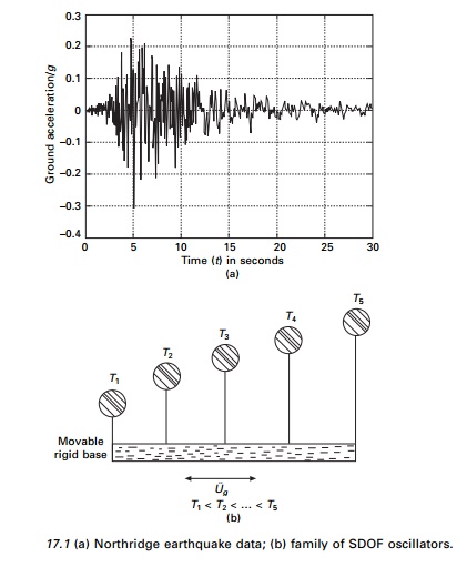
are the maximum absolute values of  relative displacement, relative velocity and total acceleration determined from Eq. 17.2, 17.6 and 17.7. However, these quantities are generally determined from numerical integration techniques. Plots of Sd, Sv, Sa versus undamped natural period of vibration for various damping ratios are called earthquake response spectra. We can construct an earthquake response spectrum, say, for Northridge earthquake (see Fig 17.1a) by considering a series of oscillators (inverted pendulums) as shown in Fig. 17.1b with varying periods of vibration attached with movable base. The base is subjected to same ground motion as that of Northridge earthquake. The maximum response for each pendulum (Sd, Sv, Sa) is plotted against the natural period for a particular value of damping. Such curves are the response spectra and are very useful for design. Figure 17.2 shows response spectra for relative displacement, relative velocity and total acceleration for the Northridge earthquake.          These quantities are generally determined by numerical evaluation using any of the numerical techniques developed in Previous Pages. Plots of Sd, Sv and S_a versus undamped natural period of vibration or natural frequency for various damping factors make up the earthquake response spectrum. The MATLAB program for drawing the spectra in Fig. 17.2 using Wilson’s recurrence formulae is shown below.

Program 17.1: MATLAB program for drawing spectra for any specified earthquake

%********************************************************** % WILSON’S RECURRENCE FORMULA TO DRAW SPECTRA FOR ANY EARTHQUAKE MOTION %**********************************************************

clc;close all;

%give initial displacement and initial velocity u(1)=0;

v(1)=0;

%tt=50 sec n=2500 for nridge %tt=30 n=1500 for elcentro ns tt=50.0;

n=2500;

n1=n+1;

dt=tt/n;

mass=1;

%**********************************************************

%      EARTHQUAKE DATA FILE FOR NORTH-RIDGE EQ IS READ FROM EXCEL DATA FILE

%      DATA FILE CONSISTS OF TIME AND THE CORRESPONDING A/G VALUES

%DATA FILE CHOPRA CONSISTS OF ELCENTRO NS DATA

EQDATA CONTAINS NORTHRIDGE DATA

%**********************************************************

de=xlsread(‘eqdata’);

%de=xlsread(‘chopra’) for i=1:n1; ug(i)=de(i,2); ug(i)=-ug(i)*9.81; p(i)=ug(i)*mass;

end;

%define damping ratios for which response is required rho=[0 0.02 0.05 .1 0.2];

for jj=1:5 r=rho(jj);

mass=1; for ii=1:200

tn=0.05*ii;

wn=2.0*pi/tn;

ss(ii)=tn;

k=mass*wn^2;

c=2.0*r*sqrt(k*mass); wd=wn*sqrt(1-r^2);

a=exp(-r*wn*dt)*(r*sin(wd*dt)/sqrt(1-r^2)+cos(wd*dt)); b=exp(-r*wn*dt)*(sin(wd*dt))/wd; c2=((1-2*r^2)/(wd*dt)-r/sqrt(1-r^2))*sin(wd*dt)-(1+2*r/(wn*dt))*cos(wd*dt); c=(1/k)*(2*r/(wn*dt)+exp(-r*wn*dt)*(c2));

d 2 = e x p ( - r * w n * d t ) * ( ( 2 . 0 * r ^ 2 - 1 ) / ( w d * d t ) * s i n ( w d * d t ) + 2 . 0 * r / (wn*dt)*cos(wd*dt));

d=(1/k)*(1-2.0*r/(wn*dt)+d2); ad=-exp(-r*wn*dt)*wn*sin(wd*dt)/(sqrt(1-r^2)); bd=exp(-r*wn*dt)*(cos(wd*dt)-r*sin(wd*dt)/sqrt(1-r^2));

c 1 = e x p ( - r * w n * d t ) * ( ( w n / s q r t ( 1 - r ^ 2 ) + r / ( d t * s q r t ( 1 - r^2)))*sin(wd*dt)+cos(wd*dt)/dt);

cd=(1/k)*(-1/dt+c1); d1=exp(-r*wn*dt)*(r*sin(wd*dt)/sqrt(1-r^2)+cos(wd*dt)); dd=(1/(k*dt))*(1-d1);

for m=2:n1 u(m)=a*u(m-1)+b*v(m-1)+c*p(m-1)+d*p(m); v(m)=ad*u(m-1)+bd*v(m-1)+cd*p(m-1)+dd*p(m); ta(m)=(-c*v(m)-k*u(m))/mass;

end dmf(ii,jj)=max(abs(u)); vmf(ii,jj)=max(abs(v)); amf(ii,jj)=max(abs(ta)); end

end

for m=1:n1 s(m)=(m-1)*dt;

end figure(1);

plot(s,ug/9.81,‘K’);

xlabel(‘ time (t) in seconds’); ylabel(‘ ground acceleration/g’); title(‘ North Ridge EQ data’); figure(2);

for ii=1:5 plot(ss,dmf(:,ii),‘K’); hold on

end

xlabel(‘ period T in seconds’);

ylabel(‘ Spectral displacement Sd in m’);

title(‘ Response spectrum for Sd North Ridge EQ)’);

legend(‘ dam=0’,‘dam=0.02’,‘dam=0.05’, ‘dam=0.1’,‘dam=0.2’) figure(3);

for ii=1:5 plot(ss,vmf(:,ii),‘K’); hold on

end

xlabel(‘ period T in seconds’);

ylabel(‘ Spectral velocity Sv in m/sec’);

title(‘ Response spectrum for Sv (North Ridge EQ)’);

legend(‘ dam=0’,‘dam=0.02’,‘dam=0.05’, ‘dam=0.1’,‘dam=0.2’) figure(4);

for ii=1:5 plot(ss,amf(:,ii)/9.81,‘K’); hold on

end

xlabel(‘ period T in seconds’);

ylabel(‘ Spectral total acceleration Sa/g’);

title(‘ Response spectrum for Sa (total) (North Ridge EQ)’); legend(‘ dam=0’,‘dam=0.02’,‘dam=0.05’, ‘dam=0.1’,‘dam=0.2’) fid=fopen(‘sv.out’,‘w’)

for jj=1:200

fprintf(fid,‘ %6.3f %6.2f %6.2f %6.2f %6.2f %6.2f\n’...

,ss(jj),vmf(jj,1),vmf(jj,2),vmf(jj,3),vmf(jj,4),vmf(jj,5)); end

fclose(fid)

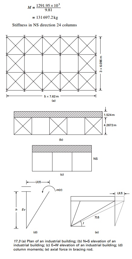
Example 17.1

An industrial building is shown in Fig. 17.3. Idealize the structure as an SDOF system. Assume the structure acts as a braced frame in the EW direction (having a total of six braced bays) and unbraced shear frame (with column base) pinned in the NS direction. Assume all columns bend about the major axis to the NS direction.

The vertical cross-bracings in the EW direction are 25.4 mm diameter steel rods. The dead weight of the structure is 1291.95 kN which is concentrated at the base of the roof trusses. Moment of inertia of columns 8.6992 × 10⁷ mm⁴. The height of the building may be assumed as 4.2672 m and the damping is 5% of critical damping. Consider Northridge earthquake.

(a)  Determine the natural period for the NS and EW directions.

(b) Conduct a time history analysis of the structure in both directions. Use the NS component of the 17 January, 1994 Northridge earthquake shown in Fig. 17.1a as input.

Solution

(a)  Natural period. Mass of the structure

(b) Time history response. The parameters in the time history response are relative displacement, u(t), relative velocity is u˙(t ), absolute total acceleration is u˙˙_t (t ). Also of interest of base shear V(t), the bending moment in columns M(t) and axial force in the steel rods T(t).

The equation of moment in NS direction

Equation of moment in EW direction

u˙˙ + 2 × 0.05 × 20 u˙ + 20 ² u = −u˙˙_g (t ) 

i.e. u˙˙ + 2 u˙ + 400 u = −u˙˙_g (t )

The value can be obtained for the Northridge earthquake by integrating above two expressions.

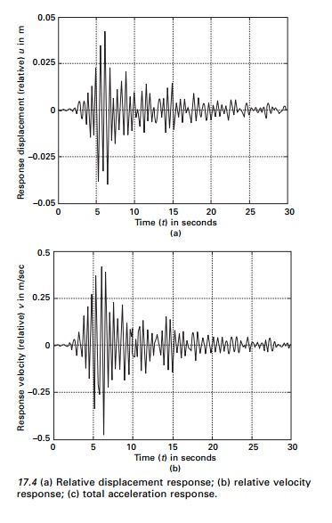
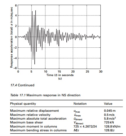
As an example. The response displacement, velocity and total acceleration are shown in Fig. 17.4 and Table 17.1 gives maximum response in NS direction.

Example 17.2

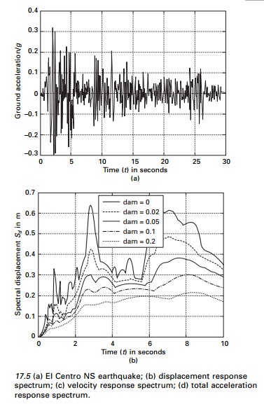
Construct response spectra for the NS component of E1 Centro earthquake (see Fig. 17.5a). Consider damping factors 0, 0.02, 0.05, 0.1 and 0.2.

Solution

The spectral displacement S_d, spectral velocity S_v and spectral acceleration S_a are determined from Eq. 17.9a, b and c respectively. The responses are evaluated numerically by direct integration of the equation

for ρ = 0.02, 0.05 and 0.1 from which maximum responses are determined. The response spectral S_d, S_v and S_a are presented in Fig. 17.5b, c and d due to the El Centro earthquake (NS) shown in Fig. 17.5a.

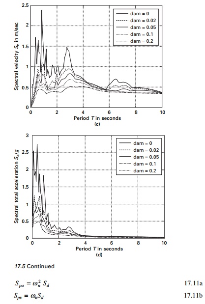
Let us define pseudo-spectral velocity and pseudo spectral acceleration as S_pv, S_pa as S_pa = ω _n² S_d = ω_n S_v; S_pv = ω_n S_d. Usually the parameters S_pv and S_pa have certain characteristics that are of practical interest. The pseudo-spectral velocity S_pv is close to spectral velocity S_v for short period structure. The comparison between S_pv and S_v for the NS component of the El Centro earthquake for ς = 0.05 is illustrated in Fig. 17.6. For zero damping, the pseudo-spectral acceleration S_pa is identical to spectral acceleration. However, for damping other than zero, the two are slightly different. Nevertheless for damping levels encountered in most engineering applications, the two can be considered practically equal.

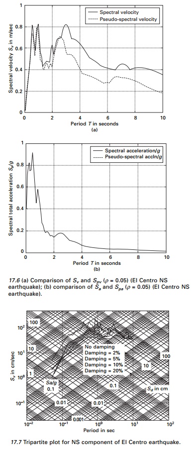
Hence the spectral relationship significantly expedites the construction of earthquake response spectra. Evaluation of spectra displacement s_d after numerical integration to obtain time history response, the corresponding pseudo spectral velocity S_pv and pseudo spectral acceleration S_pa can readily be established and we see later how s_d, s_pv and S_pa can then all be plotted on a four-way logarithmic paper.

Then for a given frequency or for a given period all the spectral quantities can be read simultaneously for the same tripartite plot. A tripartite plot of s_d,

s_pvr, S_pa for the NS component of the El Centro earthquake for various damping factors is presented in Fig. 17.7.

Program 17.2: MATLAB program to draw tripartite plot

%**********************************************************

          % to draw elastic design spectra from the earthquake data

          % read the response spectrum values in this program

          %**********************************************************

          for k=.00001:.00001:.0001

          x=0.01:1:100

          t=log(2*pi*k)-log(x)

          y=exp(t)

          loglog(x,y,‘k’),grid on

          hold on

          t=log(k*9.81/(2*pi))+log(x)

          y=exp(t)

          loglog(x,y,‘k’)

          hold on

          end

          for k=.0001:.0001:.001

          x=0.01:1:100

          t=log(2*pi*k)-log(x)

          y=exp(t)

          loglog(x,y,‘k’),grid on

          hold on

t=log(k*9.81/(2*pi))+log(x)

y=exp(t)

loglog(x,y,‘k’) hold on

end

for k=.001:.001:.01 x=0.01:1:100 t=log(2*pi*k)-log(x) y=exp(t) loglog(x,y,‘k’),grid on hold on

t=log(k*9.81/(2*pi))+log(x)

y=exp(t)

loglog(x,y,‘k’) hold on

end

xlabel(‘ period in secs’)

ylabel(‘ spectral velocity sv in cm/sec’) for k=.01:.01:.1

x=0.01:1:100 t=log(2*pi*k)-log(x) y=exp(t) loglog(x,y,‘k’),grid on hold on

t=log(k*9.81/(2*pi))+log(x)

y=exp(t)

loglog(x,y,‘k’) hold on

end

for k=.1:.1:1 x=0.01:1:100 t=log(2*pi*k)-log(x) y=exp(t) loglog(x,y,‘k’),grid on hold on

t=log(k*9.81/(2*pi))+log(x)

y=exp(t)

loglog(x,y,‘k’) hold on

end

for k=1:1:10 x=0.01:1:100 t=log(2*pi*k)-log(x) y=exp(t)

loglog(x,y,‘k’),grid on hold on

t=log(k*9.81/(2*pi))+log(x)

y=exp(t)

loglog(x,y,‘k’) hold on

end

for k=10:10:100 x=0.01:1:100 t=log(2*pi*k)-log(x) y=exp(t) loglog(x,y,‘k’),grid on hold on

t=log(k*9.81/(2*pi))+log(x)

y=exp(t)

loglog(x,y,‘k’) hold on

end

for k=100:100:1000 x=0.01:1:100 t=log(2*pi*k)-log(x) y=exp(t) loglog(x,y,‘k’),grid on hold on

t=log(k*9.81/(2*pi))+log(x)

y=exp(t)

loglog(x,y,‘k’) hold on

end

for k=1000:1000:10000 x=0.01:1:100 t=log(2*pi*k)-log(x) y=exp(t) loglog(x,y,‘k’),grid on hold on

t=log(k*9.81/(2*pi))+log(x)

y=exp(t)

loglog(x,y,‘k’) end

axis([0.01 100 0.02 500]) % d=xlsread(‘svdata’); sv=‘sv.out’

d=load(sv)

plot(d(:,1),100*d(:,2),‘k’)

plot(d(:,1),100*d(:,3),‘k’)

plot(d(:,1),100*d(:,4),‘k’)

plot(d(:,1),100*d(:,5),‘k’)

plot(d(:,1),100*d(:,6),‘k’)

text(0.2,0.02,‘0.001’);

text(0.6,0.1,‘0.01’);

text(2,0.3,‘0.1’);

text(7,1,‘1’);

text(20,3,‘10’);

text(80,10,‘100’) text(20,1,‘sd in cm’) xlabel(‘ period in sec’) ylabel(‘ sv in cm/sec’) text(0.01,200,‘100’) text(0.01,20,‘10’) text(0.01,2,‘1’) text(0.02,0.4,‘0.1’) text(0.07,0.1,‘0.01’) text(.02,0.8,’sa/g’) gtext(‘ no damping’) gtext(‘ damping=2%’) gtext(‘ damping=5%’) gtext(‘ damping=10%’) gtext(‘ damping=20%’)