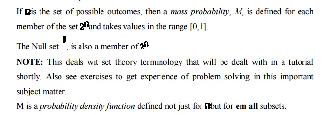
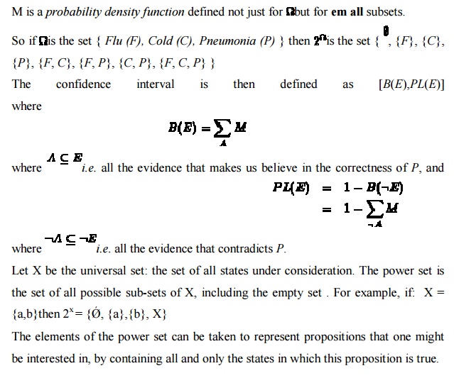
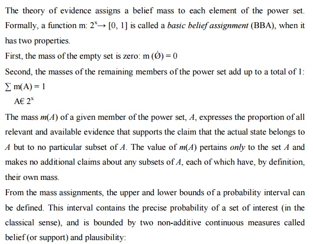
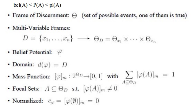
Chapter: Artificial Intelligence
Dempster- Shafer theory
Dempster- Shafer theory
The Dempster-Shafer theory, also known as the
theory of belief functions, is a generalization of the Bayesian theory of
subjective probability.
Whereas the Bayesian theory requires probabilities
for each question of interest, belief functions allow us to base degrees of
belief for one question on probabilities for a related question. These degrees
of belief may or may not have the mathematical properties of probabilities;
The Dempster-Shafer theory owes its name to work by
A. P. Dempster (1968) and Glenn Shafer (1976), but the theory came to the
attention of AI researchers in the early 1980s, when they were trying to adapt
probability theory to expert systems.
Dempster-Shafer degrees of belief resemble the
certainty factors in MYCIN, and this resemblance suggested that they might
combine the rigor of probability theory with the flexibility of rule-based
systems.
The Dempster-Shafer theory remains attractive
because of its relative flexibility. The Dempster-Shafer theory is based on two
ideas: the idea of obtaining degrees of belief for one question from subjective
probabilities for a related question,
Dempster's rule for combining such degrees of
belief when they are based on independent items of evidence.
To illustrate the idea of obtaining degrees of
belief for one question from subjective probabilities for another, suppose I
have subjective probabilities for the reliability of my friend Betty. My
probability that she is reliable is 0.9, and my probability that she is
unreliable is 0.1. Suppose she tells me a limb fell on my car. This statement,
which must true if she is reliable, is not necessarily false if she is
unreliable. So her testimony alone justifies a 0.9 degree of belief that a limb
fell on my car, but only a zero degree of belief (not a 0.1 degree of belief)
that no limb fell on my car. This zero does not mean that I am sure that no
limb fell on my car, as a zero probability would; it merely means that Betty's
testimony gives me no reason to believe that no limb fell on my car. The 0.9
and the zero together constitute a belief function.
To illustrate Dempster's rule for combining degrees
of belief, suppose I also have a subjective probability for the reliability of
Sally, and suppose she too testifies, independently of Betty, that a limb fell
on my car. The event that Betty is reliable is independent of the event that
Sally is reliable, and we may multiply the probabilities of these events; the
probability that both are reliable is 0.9x0.9 = 0.81, the probability that neither
is reliable is 0.1x0.1 = 0.01, and the probability that at least one is
reliable is 1 - 0.01 = 0.99. Since they both said that a limb fell on my car,
at least of them being reliable implies that a limb did fall on my car, and
hence I may assign this event a degree of belief of 0.99. Suppose, on the other
hand, that Betty and Sally contradict each other—Betty says that a limb fell on
my car, and Sally says no limb fell on my car. In this case, they cannot both
be right and hence cannot both be reliable—only one is reliable, or neither is
reliable. The prior probabilities that only Betty is reliable, only Sally is
reliable, and that neither is reliable are 0.09, 0.09, and 0.01, respectively,
and the posterior probabilities (given that not both are reliable) are 9 19 , 9
19 , and 1 19 , respectively. Hence we have a 9 19 degree of belief that a limb
did fall on my car (because Betty is reliable) and a 9 19 degree of belief that
no limb fell on my car (because Sally is reliable).
In summary, we obtain degrees of belief for one
question (Did a limb fall on my car?) from probabilities for another question
(Is the witness reliable?). Dempster's rule begins with the assumption that the
questions for which we have probabilities are independent with respect to our subjective
probability judgments, but this independence is only a priori; it disappears
when conflict is discerned between the different items of evidence.
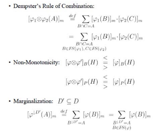
Implementing the Dempster-Shafer theory in a
specific problem generally involves solving two related problems.
First, we must sort the uncertainties in the
problem into a priori independent items of evidence.
Second, we must carry out Dempster's rule
computationally. These two problems and their solutions are closely related.
Sorting the uncertainties into independent items
leads to a structure involving items of evidence that bear on different but
related questions, and this structure can be used to make computations
This can be regarded as a more general approach to
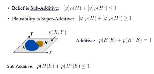
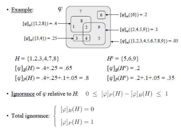
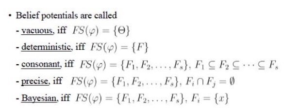
representing uncertainty than the Bayesian approach.
The basic idea in representing uncertainty in this
model is:
The belief brings together all the evidence that would lead us to believe in P with some certainty.
The plausibility brings together the evidence that is compatible with P and is not inconsistent with it.
This method allows for further additions to the set of knowledge and does not assume disjoint outcomes.
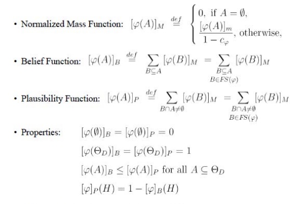
Benefits of Dempster-Shafer Theory:
Allows proper distinction between reasoning and
decision taking
No modeling restrictions (e.g. DAGs)
It represents properly partial and total ignorance
Ignorance is quantified:
low degree of ignorance means
high confidence in results
enough information available for taking decisions
high degree of ignorance means
low confidence in results
gather more information (if possible) before taking
decisions
Conflict is quantified:
low conflict indicates the presence of confirming
information sources
high conflict indicates the presence of
contradicting sources
Simplicity: Dempster’s rule of combination covers
combination of evidence
Bayes’ rule
Bayesian updating (conditioning)
belief revision (results from non-monotonicity)
DS-Theory is not very successful because:
Inference is less efficient than Bayesian inference
Pearl is the better speaker than Dempster (and
Shafer, Kohlas, etc.)
Microsoft supports Bayesian Networks
The UAI community does not like „outsiders“
Related Topics