Chapter: Artificial Intelligence(AI) : Planning and Machine Learning
Dempster - Shafer Theory (DST)
Dempster ŌĆō Shafer Theory (DST)
DST is a mathematical theory of evidence based on belief functions and plausible reasoning. It is used to combine separate pieces of information (evidence) to calculate the probability of an event.
DST offers an alternative to
traditional probabilistic theory for the mathematical representation of uncertainty.
DST can be regarded as, a more
general approach to represent uncertainty than the Bayesian approach.
Bayesian methods are sometimes
inappropriate
Example :
Let A represent the proposition "Moore is attractive". Then the axioms of probability
insist that P(A) + P(¬A) = 1.
Now suppose that Andrew does not
even know who "Moore" is, then
We cannot say that Andrew
believes the proposition if he has no idea what it means.
Also, it is not fair to say that
he disbelieves the proposition.
It would therefore be meaningful
to denote Andrew's belief B of
B(A) and B(¬A) as
both being 0.
Certainty factors do not allow
this.
Dempster-Shafer Model
The
idea is to allocate a
number between 0 and 1 to indicate a degree of belief on a proposal as in the probability framework.
However, it is not considered a
probability but a belief mass. The distribution of
masses is called basic belief assignment.
In other words, in this formalism a
degree of belief (referred as mass)
is represented as a belief
function rather than a Bayesian probability distribution.
Example: Belief assignment (continued from previous slide)
Suppose a system has five
members, say five independent states, and exactly one of which is actual. If
the original set is called S, | S | = 5, then
the set of all subsets (the power
set) is called 2S.
If each possible subset as a
binary vector (describing any member is present or not by writing 1
or 0
), then 25 subsets are possible, ranging from the empty subset ( 0, 0, 0, 0, 0 ) to the "everything" subset ( 1, 1,
1, 1, 1 ).
The "empty" subset represents a "contradiction", which is not true in any state,
and is thus assigned a mass of one ;
The remaining masses are normalized so that
their total is 1.
The "everything" subset is labeled as
"unknown"; it represents the state
where all elements are present one ,
in the sense that you cannot tell which is actual.
Belief and Plausibility
Shafer's framework allows for
belief about propositions to be represented as intervals, bounded by two
values, belief (or support) and plausibility:
belief Ōēż plausibility
Belief in a hypothesis is
constituted by the sum of the masses of all
sets enclosed by it (i.e. the sum
of the masses of all subsets of the hypothesis). It is the amount of belief
that directly supports a given hypothesis at least in part, forming a lower
bound.
Plausibility is 1 minus the sum of the masses of all sets whose intersection with the hypothesis is empty. It is an
upper bound on the possibility that the hypothesis could possibly happen, up to
that value, because there is only so much evidence that contradicts that
hypothesis.
Example :
A proposition say "the
cat in the box is dead."
Suppose we have belief of 0.5 and plausibility of 0.8 for the proposition.
Example :
Suppose we have belief of 0.5 and plausibility of 0.8 for the proposition.
Evidence to state strongly, that
proposition is true with confidence 0.5. Evidence contrary to hypothesis
("the cat is alive") has confidence 0.2.
Remaining mass of 0.3
(the gap between the 0.5 supporting evidence and the 0.2
contrary evidence) is "indeterminate," meaning that the
cat could either be dead or
alive. This interval represents the level of uncertainty based on the evidence
in the system.
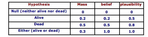
Null hypothesis is set to zero
by definition, corresponds to "no solution". Orthogonal hypotheses
"Alive" and "Dead" have probabilities of 0.2
and
0.5,
respectively. This could correspond to "Live/Dead Cat Detector"
signals, which have respective
reliabilities of 0.2 and 0.5. All-encompassing
"Either" hypothesis (simply acknowledges there is a cat in the box)
picks up the slack so that the sum of the masses is 1. Belief for the "Alive" and "Dead"
hypotheses matches their corresponding masses because they have no subsets;
Belief for "Either"
consists of the sum of all three masses (Either, Alive, and Dead) because
"Alive" and "Dead" are each subsets of "Either".
"Alive" plausibility is
1- m (Death) and "Dead" plausibility is 1- m
(Alive). "Either" plausibility sums m(Alive) + m(Dead) + m(Either).
Universal hypothesis
("Either") will always have 100% belief and plausibility; it acts
as a checksum of sorts.
Dempster-Shafer Calculus
In the previous slides, two
specific examples of Belief and plausibility have been stated. It would now be
easy to understand their generalization.
The Dempster-Shafer (DS) Theory,
requires a Universe of Discourse U (or Frame of Judgment) consisting of mutually exclusive
alternatives, corresponding to an attribute value domain. For instance, in
satellite image classification the set U may consist of all possible classes of
interest.
Each subset S ŌŖå
U is assigned a basic probability
m(S), a belief Bel(S), and a plausibility Pls(S) so that m(S),
Bel(S), Pls(S) Ōłł [0, 1] and
Pls(S) Ōēź Bel(S) where
m represents the strength of an
evidence, is the basic probability;
e.g., a group of pixels belong to
certain class, may be assigned value m.
Bel(S) summarizes all the reasons
to believe S.
Pls(S) expresses how much one
should believe in S if all currently unknown facts were to support S.
The true belief in S is somewhere
in the belief interval [Bel(S), Pls(S)].
The basic probability assignment m
is defined as function
m : 2U ŌåÆ [0,1] , where m(├ś) = 0 and sum of m over all subsets of
U is 1 (i.e., Ōłæ S ŌŖå U
m(s) = 1 ).
For a given
basic probability assignment
m, the belief Bel of a subset A of U is the sum of m(B) for all subsets
B of A , and the plausibility Pls of a subset A
of U is Pls(A) = 1 - Bel(A') (5)
where A' is complement of A in U.
Summarize :
The confidence interval is that
interval of probabilities within which the true probability lies with a certain
confidence based on the belief "B" and plausibility "PL"
provided by some evidence "E" for a proposition "P".
The belief brings together all the
evidence that would lead us to believe in the proposition P with some
certainty.
The plausibility brings together
the evidence that is compatible with the proposition P and is not inconsistent
with it.
If "Ōä”" is the set of
possible outcomes, then a mass probability "M" is defined for each
member of the set 2Ōä” and takes values in the range [0,1] . The Null set,
"čä", is also a member of 2Ōä” .
Example
If Ōä” is the set { Flu (F), Cold
(C), Pneumonia (P) }
Then 2Ōä” is the set Confidence
interval is {čä, {F}, {C}, {P}, {F, C}, {F, P}, {C, P}, {F, C, P}} then defined
as where
B(E) = ŌłæA M , where A ŌŖå E
i.e., all evidence that makes us believe in the correctness of P, and
PL(E) = 1 ŌĆō B(┬¼E) = Ōłæ┬¼A M , where
┬¼A ŌŖå ┬¼E i.e., all the evidence that
contradicts P.
Combining Beliefs
The Dempster-Shafer calculus
combines the available evidences resulting in a belief and a plausibility in
the combined evidence that represents a consensus on the correspondence. The
model maximizes the belief in the combined evidences.
The rule of combination states that two basic probability assignments M1 and
M2 are combined into a by third basic probability assignment the normalized
orthogonal sum m1 (+) m2 stated below.
Suppose M1 and M2 are two belief
functions.
Let X be the set of subsets of Ōä” to
which M1 assigns a nonzero value and let Y be a similar set for M2 , then a new
belief function M3 from the combination of beliefs in M1 and M2 is obtained as
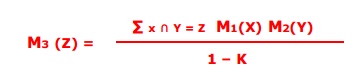
where Ōłæ x Ōł® Y = čä M1(X) M2(Y) , for Z = čä
M3 (čä) is
defined to be 0 so that the orthogonal sum remains a
basic probability assignment.
Related Topics