Production System

Production System

Types of Production Systems.

A Knowledge representation formalism consists of collections of condition-action rules(Production Rules or Operators), a database which is modified in accordance with the rules, and a Production System Interpreter which controls the operation of the rules i.e The 'control mechanism' of a Production System, determining the order in which Production Rules are fired.

A system that uses this form of knowledge representation is called a production system.

A production system consists of rules and factors. Knowledge is encoded in a declarative from which comprises of a set of rules of the form

Situation ------------ Action SITUATION that implies ACTION.

Example:-

IF the initial state is a goal state THEN quit.

The major components of an AI production system are

A global database

A set of production rules and

A control system

The goal database is the central data structure used by an AI production system. The production system. The production rules operate on the global database. Each rule has a precondition that is either satisfied or not by the database. If the precondition is satisfied, the rule can be applied. Application of the rule changes the database. The control system chooses which applicable rule should be applied and ceases computation when a termination condition on the database is satisfied. If several rules are to fire at the same time, the control system resolves the conflicts.

Four classes of production systems:-

A monotonic production system

A non monotonic production system

A partially commutative production system

A commutative production system. Advantages of production systems:-

Production systems provide an excellent tool for structuring AI programs.

Production Systems are highly modular because the individual rules can be added, removed or modified independently.

The production rules are expressed in a natural form, so the statements contained in the knowledge base should the a recording of an expert thinking out loud.

Disadvantages of Production Systems:-

One important disadvantage is the fact that it may be very difficult analyse the flow of control within a production system because the individual rules don’t call each other.

Production systems describe the operations that can be performed in a search for a solution to the problem. They can be classified as follows.

Monotonic production system :- A system in which the application of a rule never prevents the later application of another rule, that could have also been applied at the time the first rule was selected.

Partially commutative production system:-

A production system in which the application of a particular sequence of rules transforms state X into state Y, then any permutation of those rules that is allowable also transforms state x into state Y.

Theorem proving falls under monotonic partially communicative system. Blocks world and 8 puzzle problems like chemical analysis and synthesis come under monotonic, not partially commutative systems. Playing the game of bridge comes under non monotonic , not partially commutative system.

For any problem, several production systems exist. Some will be efficient than others. Though it may seem that there is no relationship between kinds of problems and kinds of production systems, in practice there is a definite relationship.

Partially commutative , monotonic production systems are useful for solving ignorable problems. These systems are important for man implementation standpoint because they can be implemented without the ability to backtrack to previous states, when it is discovered that an incorrect path was followed. Such systems increase the efficiency since it is not necessary to keep track of the changes made in the search process.

Monotonic partially commutative systems are useful for problems in which changes occur but can be reversed and in which the order of operation is not critical (ex: 8 puzzle problem).

Production systems that are not partially commutative are useful for many problems in which irreversible changes occur, such as chemical analysis. When dealing with such systems, the order in which operations are performed is very important and hence correct decisions have to be made at the first time itself.

Control or Search Strategy :

Selecting rules; keeping track of those sequences of rules that have already been tried and the states produced by them.

Goal state provides a basis for the termination of the problem solving task.

PATTERN MATCHING STAGE

Execution of a rule requires a match.

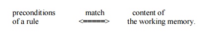
when match is found => rule is applicable several rules may be applicable

CONFLICT RESOLUTION (SELECTION STRATEGY ) STAGE

Selecting one rule to execute;

ACTION STAGE

Applying the action part of the rule => changing the content of the workspace =>new patterns,new matches => new set of rules eligible for execution Recognize -act control cycle

Search Strategies

Uninformed Search Strategies have no additional information about states beyond that

provided in the problem definition.

Strategies that know whether one non goal state is ―more promising‖ than another are

called Informed search or heuristic search strategies. There are five uninformed search strategies as given below. o Breadth-first search

Uniform-cost search o Depth-first search

Depth-limited search

Iterative deepening search

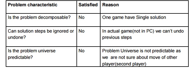
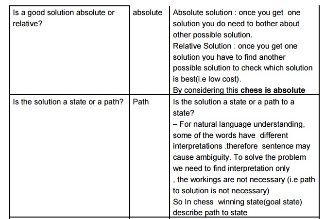
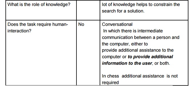
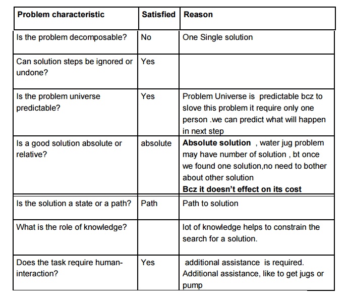
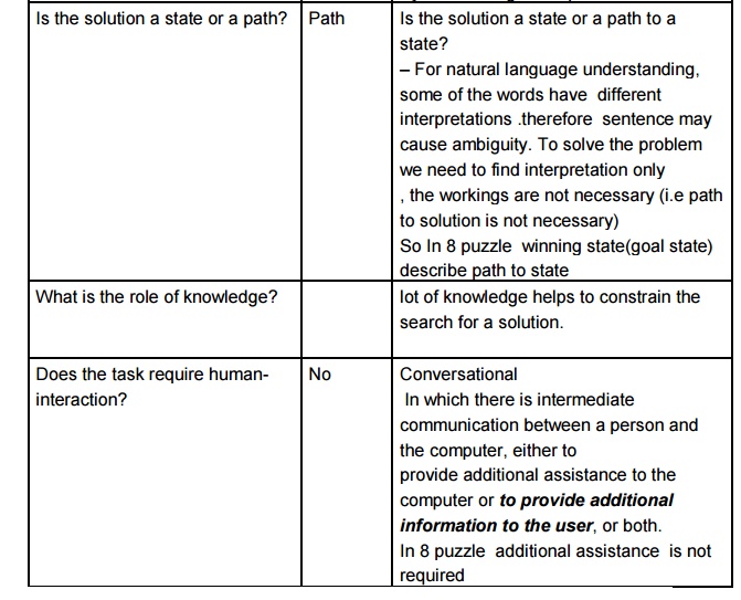
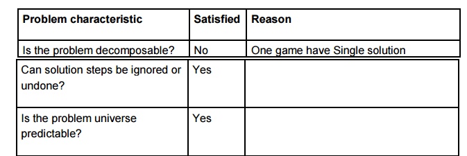
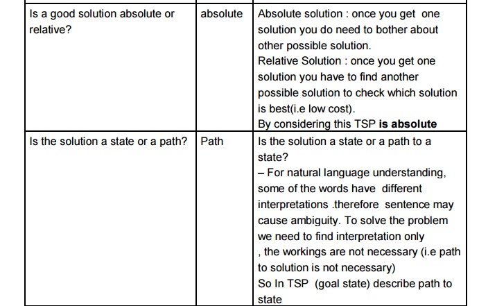
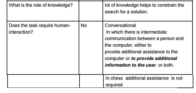
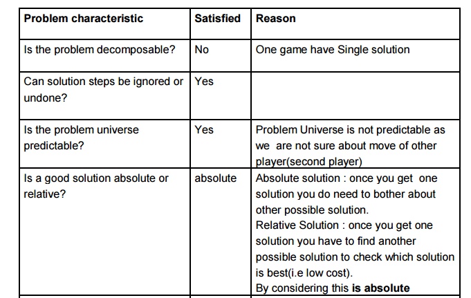
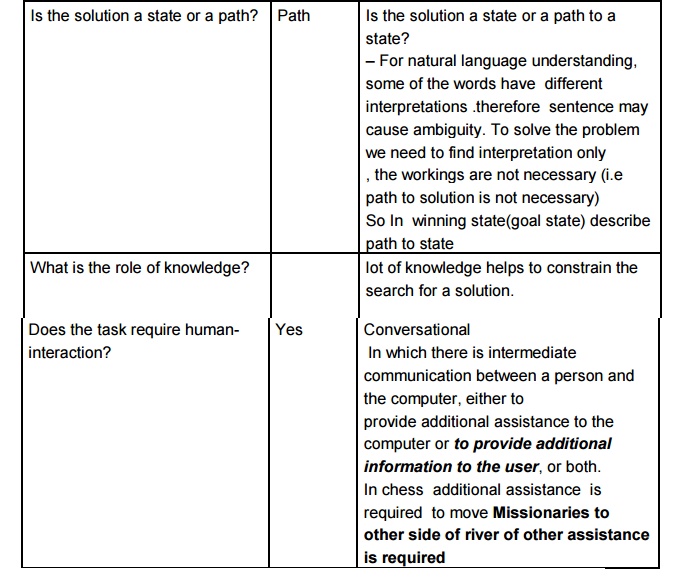
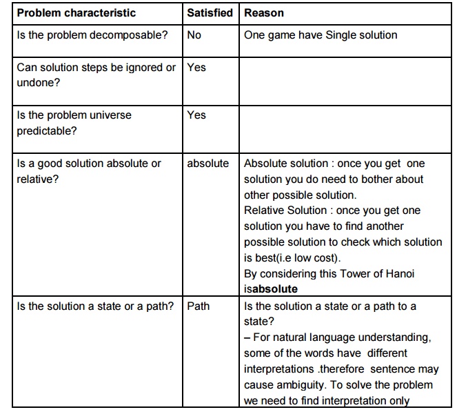
Problem characteristics

Analyze each of them with respect to the seven problem characteristics

Chess

Water jug

8-puzzle

Traveling salesman

Missionaries and cannibals

Tower of Hanoi

Chess

Water jug

8 puzzle

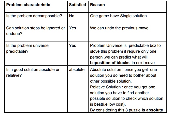
Travelling Salesman (TSP)

Missionaries and cannibals

Tower of Hanoi

Measuring Performance of Algorithms

There are two aspects of algorithmic performance:

Time

Instructions take time.

How fast does the algorithm perform?

What affects its runtime?

Space

- Data structures take                     space

What kind of data structures can be used?

How does choice of data structure affect the runtime?

Algorithms can not be compared by running them on computers. Run time is system dependent. Even on same computer would depend on language Real time units like microseconds not to be used.

Generally concerned with how the amount of work varies with the data.

Measuring Time Complexity

Counting number of operations involved in the algorithms to handle n items.

Meaningful comparison for very large values of  n.

Complexity of Linear Search

Consider the task of searching a list to see if it contains a particular value.

A useful search algorithm should be general.

Work done varies with the size of the list

What can we say about the work done for list of any length?

i = 0;

while (i < MAX && this_array[i] != target) i = i + 1;

if (i <MAX)

printf ( “Yes, target is there \n” ); else

printf( “No, target isn’t there \n” );

The work involved : Checking target value with each of the n elements.

no. of operations: 1        (best case)

n        (worst case)

n/2     (average case)

Computer scientists tend to be concerned about the Worst Case complexity.

The worst case guarantees that the performance of the algorithm will be at least as good as the analysis indicates.

Average Case Complexity:

It is the best statistical estimate of actual performance, and tells us how well an algorithm performs if you average the behavior over all possible sets of input data. However, it requires considerable mathematical sophistication to do the average case analysis.

Algorithm Analysis: Loops

Consider an n X n two dimensional array. Write a loop to store the row sums in a one-dimensional array rows and the overall total in grandTotal.

LOOP 1:

grandTotal = 0;

for (k=0; k<n-1; ++k) { rows[k] = 0;

for (j = 0; j <n-1; ++j){

rows[k] = rows[k] + matrix[k][j]; grandTotal = grandTotal + matrix[k][j];

}

}

It takes 2n² addition operations

LOOP 2:

grandTotal =0;

for (k=0; k<n-1; ++k) rows[k] = 0;

for (j = 0; j <n-1; ++j)

rows[k] = rows[k] + matrix[k][j]; grandTotal = grandTotal + rows[k];

}

This one takes n²  + n operations

Big-O Notation

We want to understand how the performance of an algorithm responds to changes in problem size. Basically the goal is to provide a qualitative insight. The Big-O notation is a way of measuring the order of magnitude of a mathematical expression

O(n) means on the Order of n

Consider

n⁴ + 3₁n² + 10  = f (n)

The idea is to reduce the formula in the parentheses so that it captures the qualitative behavior in simplest possible terms. We eliminate any term whose contribution to the total ceases to be significant as n becomes large.

We also eliminate any constant factors, as these have no effect on the overall pattern as n increases. Thus we may approximate f(n) above as

(n⁴ + 3₁n² + 10) = O( n⁴⁾

Let g(n) = n⁴

Then the order of f(n) is O[g(n)].

Definition: f(n) is O(g(n)) if there exist positive numbers c and N such that f(n) < = c g(n) for all n >=N.

i.e. f is big –O of g if there is larger than cg for sufficiently large than N) such that f is not value of n ( greater  c g(n) is an upper bound on the value of f(n)

That is, the number of operations is at worst proportional to g(n) for all large values of n.

How does one determine c and N?

Let f(n) = 2 n² + 3 n + 1  = O (n² )

Now 2 n² + 3 n + 1 < = c n²

Or 2 + (3/n) + ( 1 / n²  ) < = c

You want to find c such that a term in f becomes the largest and stays the largest. Compare first and second term. First will overtake the second at N = 2,

so for N= 2, c >= 3.75,

for N = 5, c >= slightly more than 2, for very large value of n, c is almost 2.

g is almost always > = f if it is multiplied by a constant c

Look at it another way : suppose you want to find weight of elephants, cats and ants in a jungle. Now irrespective of how many of each item were there, the net weight would be proportional to the weight of an elephant.

Incidentally we can also say f is big -O not only of  n²

but also of n³  , n⁴   , n⁵  etc (HOW ?)

­ Loop 1 and Loop 2 are both in the same big-O category: O(n²)

Properties of Big-O notation:

O(n) + O(m) = O(n) if n > = m

The function log n to base a is order of O( log n to base b) For any values of a and b ( you can show that any log values are multiples of each other)

Linear search Algorithm:

Best Case - It’s the first value “order 1,” O(1)

Worst Case - It’s the last value, n “order n,” O(n)

Average - N/2 (if value is present) “order n,” O(n)

Example 1:

Use big-O notation to analyze the time efficiency of the following fragment of C code:

for(k = 1; k <= n/2; k++)

{

.

.

for (j = 1; j <= n*n; j++)

{

}

}

Since these loops are nested, the efficiency is n³/2, or O(n³) in big-O terms.

Thus, for two loops with O[f₁(n)] and O[f₂(n)] efficiencies, the efficiency of the nesting of these two loops is

O[f₁(n) * f₂(n)].

Example 2:

Use big-O notation to analyze the time efficiency of the following fragment of C code:

for (k=1; k<=n/2; k++)

{

.

.

}

for (j = 1; j <= n*n; j++)

{

.

.

}

The number of operations executed by these loops is the sum of the individual loop efficiencies. Hence, the efficiency is n/2+n², or O(n²) in big-O terms.

Thus, for two loops with O[f₁(n)] and O[f₂(n)] efficiencies, the efficiency of the sequencing of these two loops is O[f_D(n)] where f_D(n) is the dominant of the functions f₁(n) and f₂(n).

Complexity of Linear Search

In measuring performance, we are generally concerned with how the amount of work varies with the data. Consider, for example, the task of searching a list to see if it contains a particular value.

A useful search algorithm should be general.

Work done varies with the size of the list

What can we say about the work done for list of any length?

i = 0;

while (i < MAX && this_array[i] != target) i = i + 1;

if (i <MAX)

printf ( “Yes, target is there \n” ); else

printf( “No, target isn’t there \n” );

Order Notation

How much work to find the target in a list containing N elements?

Note: we care here only about the growth rate of work. Thus, we toss out all constant values.

Best Case work is constant; it does not grow with the size of the list.

Worst and Average Cases work is proportional to the size of the list, N.

Order Notation

O(1) or “Order One”: Constant time

does not mean that it takes only one operation

does mean that the work doesn’t change as N changes is a notation for “constant work”

O(n) or “Order n”: Linear time

does not mean that it takes N operations

does mean that the work changes in a way that is proportional to N

is a notation for “work grows at a linear rate”

O(n²) or “Order n² ”: Quadratic time

O(n³) or “Order n³ ”: Cubic time

Algorithms whose efficiency can be expressed in terms of a polynomial of the form

a_mn^m + a_m-1n^m-1 + ... + a₂n² + a₁n + a₀

are called polynomial algorithms. Order O(n^m).

Some algorithms even take less time than the number of elements in the problem. There is a notion of logarithmic time algorithms.

We know 10³  =1000

So we can write it as log₁₀1000 = 3

Similarly suppose we have

2⁶  =64

then we can write

log₂64 = 6

If the work of an algorithm can be reduced by half in one step, and in k steps we are able to solve the problem then

2^k  = n

or in other words

log₂n = k

This algorithm will be having a logarithmic time complexity ,usually written as O(ln n).

Because log_an will increase much more slowly than n itself, logarithmic algorithms are generally very efficient. It also can be shown that it does not matter as to what base value is chosen.

Example 3:

Use big-O notation to analyze the time efficiency of the following fragment of C code:

k = n;

while (k > 1)

{

.

.

k = k/2;

}

Since the loop variable is cut in half each time through the loop, the number of times the statements inside the loop will be executed is log₂n.

Thus, an algorithm that halves the data remaining to be processed on each iteration of a loop will be an O(log₂n) algorithm.

There are a large number of algorithms whose complexity is O( n log₂n) .

Finally there are algorithms whose efficiency is dominated by a term of the form aⁿ

These are called exponential algorithms. They are of more theoretical rather than practical interest because they cannot reasonably run on typical computers for moderate values of n.

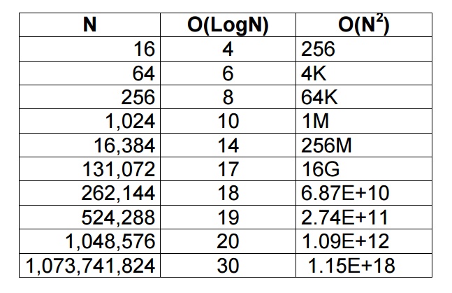
Comparison of N, logN and N²

Constraint Satisfaction

Constraint satisfaction is the process of finding a solution to a set of constraints that impose conditions that the variables must satisfy. A solution is therefore a set of values for the variables that satisfies all constraints—that is, a point in the feasible region.

The techniques used in constraint satisfaction depend on the kind of constraints being considered. Often used are constraints on a finite domain, to the point that constraint satisfaction problems are typically identified with problems based on constraints on a finite domain. Such problems are usually solved via search, in particular a form of backtracking or local search. Constraint propagation are other methods used on such problems; most of them are incomplete in general, that is, they may solve the problem or prove it unsatisfiable, but not always. Constraint propagation methods are also used in conjunction with search to make a given problem simpler to solve. Other considered kinds of constraints are on real or rational numbers; solving problems on these constraints is done via variable elimination or the simplex algorithm.

Complexity

Solving a constraint satisfaction problem on a finite domain is an NP complete problem with respect to the domain size. Research has shown a number of tractable subcases, some limiting the allowed constraint relations, some requiring the scopes of constraints to form a tree, possibly in a reformulated version of the problem. Research has also established relationship of the constraint satisfaction problem with problems in other areas such as finite model theory.