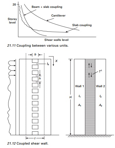
Coupled shear walls

Coupled shear walls

When two or more shear walls are connected by a system of beams or slabs, total stiffness exceeds the summation of individual stiffness. This is because the connecting beam restrains individual cantilever action. Shear walls resist lateral forces up to 30–40 storeys (see Fig. 21.10). Walls with openings present a complex problem to the analyst.

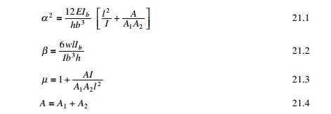
Openings normally occur in vertical rows throughout the height of the wall and the connection between wall cross-sections is provided either by connecting beams which form part of the wall or floor slab or a combination of both. The terms ‘coupled shear walls’, ‘pierced shear walls’ and ‘shear wall with openings’ are commonly described for such units. If the openings are very small, their effect on the overall state of stress in the shear wall is minimal. Large openings have a pronounced effect and if large enough result in a system in which frame action predominates. The degree of coupling between two walls separated by a row of openings has been expressed of geometric parameter α (having a unit of 1/length) which it gives a measure of relative stiffness of beams with respect to that of walls. When αH exceeds 13, the walls may be analysed as a single homogenous cantilever. When αH<0.8 the wall may be analysed as the separate cantilever, 0.8<αH<13, the

stiffness of connecting beam must be considered. The effectiveness of coupling can clearly be seen in Fig. 21.11.

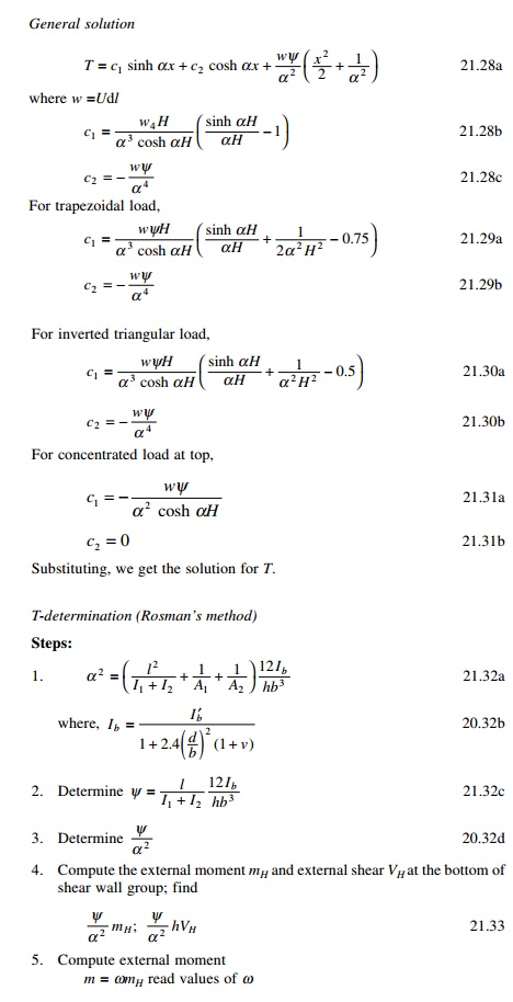
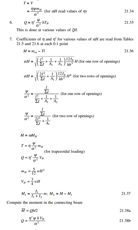
1.Continuous medium method due to Rosman (1966)

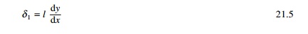
The individual connecting beams of finite stiffness Ib are replaced by an imaginary continuous connection or lamina. The equivalent stiffness of the lamina for a storey height h is Ib/h, giving stiffness of Ib/h dx for a height of dx (see Fig. 21.12).

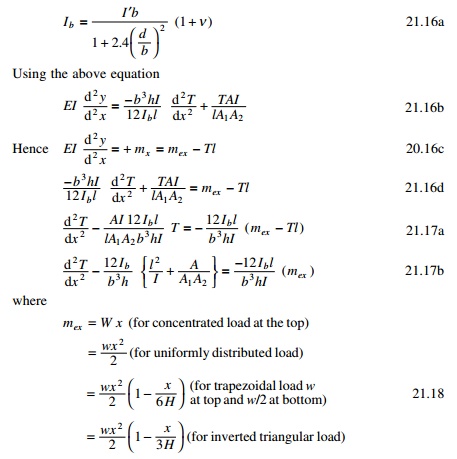
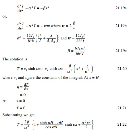
When the wall is subjected to horizontal loading, the walls deflect, inducing vertical shear force in the laminas. The system is made statically determinate by introducing a cut along a centre line of beams, which is assumed to lie on the points of contra-flexure. The displacement at each wall is determined and by considering the compatibility of deformation of the lamina, a second order differential equation with the vertical shear force as a variable is established. The solution of the differential equations with fixed base boundary conditions is most common loading to an equation for the integral shear T from which the moment, axial loads in the walls can be established and all the other quantities can be written.

E       –        Modulus of elasticity

b        –        Width of opening

Ab     –        Area of connecting beam

I        –        I1 + I2

G       –        Shear modulus

Ib      –        Moment of inertia of connecting beam including shear deformation

d        –        depth of inter-connecting beam

ν   –  Poisson’s ratio

α, β, β, are the parameters given by following equations:

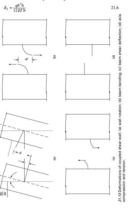
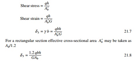
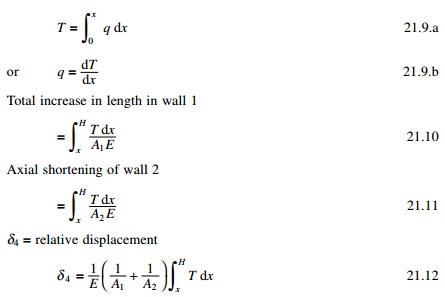
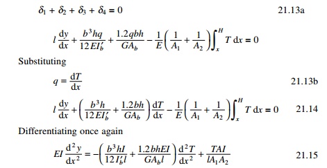
Under lateral loads the two ends of the beam experience a vertical displacement consisting of contributions δ1, δ2, δ3 and δ4 as shown in Fig. 21.13

Wall rotation

The relative displacement δ1 due to bending of each wall element is given by

Beam bending

The shear force V = qh acting at each floor level at the centre of connecting beams with centre relations displacement δ2

Beam shear deflection                                                   

The same shear force causes a deformation δ3 as

Axial compression and tension

The displacement δ4 is the relative displacement of the two wall elements due to axial deformations of the walls caused by T acting as a vertical wall on the wall elements

Since the two walls are connected, the compatability and stipulation that the relative displacement vanishes

The first two terms on the right-hand side of the above equation which pertain to bending and shear deflection of the beam and can be combined to a single term by reducing moment of inertia to include shear deformation as

2 Coupled shear wall subjected to uniformly distributed load)

Once the distribution of force T has been obtained the shear force in the coupling beam may be determined as the difference in values of T at levels h/2 above below and above that level

The general expression for deflection y at a point x can  be obtained by integrating with the expression

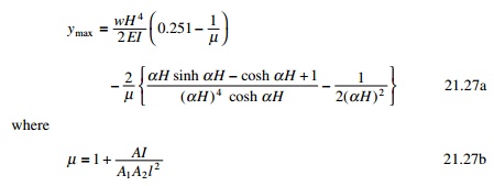
where H is measured from the top. Although inter-storey drifts are important most usually in preliminary analysis, the maximum deflection at the top is of prime interest. This is given by the following expression

To analyse a system of coupled shear wall by the method requires laborious calculation. Several researchers have proposed simplified procedures. Coull and Choudhury (1967) proposed the following method. The stress distribution of coupled shear walls is obtained as a combination of two distinct actions.

1.     Walls acting together as a single composite cantilever with neutral axis located at the centroid of two elements.

2.     Walls acting as two independent cantilever bending about their neutral axis. Semi-graphical methods are also presented for rapid design.

Example 21.2

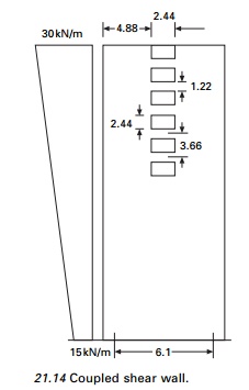
Analyse the shear wall shown in Fig. 21.14. Thickness of wall = 300 mm; width of I wall = 4.88 m; width of II wall = 2.44 m  Width of opening = 2.44m.

Solution

Total width = 4.88 + 4.88 = 9.76

I = 2.44+ 2.44+ 1.22 = 6.1 m

b = 2.44 m d = 1.22 m

H = 73.152 m h = 3.66 m

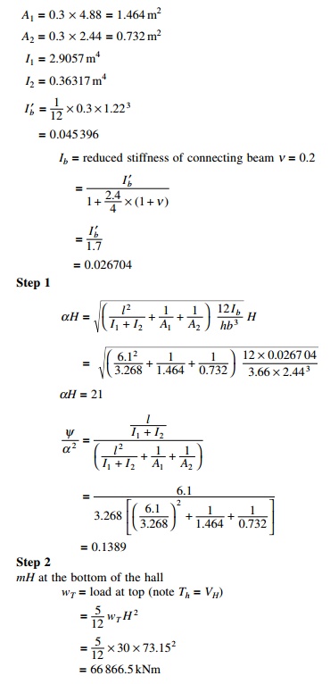
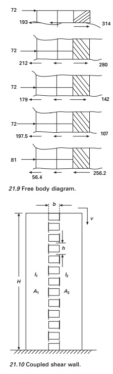
The calculations for the variations of moments, T, in the walls and the moment in the connecting beam are shown in Table 21.7 and the moments in both the walls, the moment in the link beam and T in the walls are shown in Fig. 21.15.

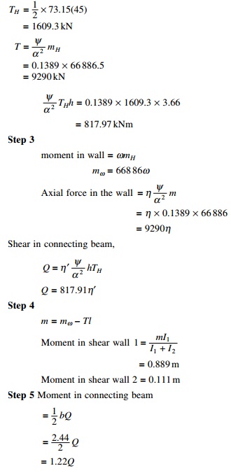
Coupled shear walls with two rows of openings are shown in Fig. 21.16.

Program 21.1 MATHEMATICA program for coupled shear wall

The program is executed in MATHEMATICA and the variation of moment in wall 1, moment in wall 2, moment in link beam and T of the wall are as shown in Fig. 20.15 for the coupled shear wall of height 73.15 m with width of the walls 4.88 and 2.44 m and thickness of the wall 0.3 m, width and depth of opening as 2.44 m, depth of link beam as 1.22 m and centre to centre of the wall as 6.1 m subjected to trapezoidal load of 30 k/m at the top and 15 kN/m at the bottom. Young’s modulus and Poisson’s ratio may be assumed as 20 GPa and 0.2 respectively. For the problem considered α2 = 0.08237; ψ = 00114; c2 = 15; c3= –0.0346. The program in MATHEMATICA is shown on page 859.

DSolve[{T’’[x]-0.08237*T[x]==-0.0114*(15*x^2-0.0346*x^3),T[0]==T’[73.15]==0},T[x],x]

.

T=T[x]

t = –6.01903 ×  10–7e–0.287002x(8.37456 ×  107

–8.37456 ×  107e0.287002x  + 1.e0.574003x

–579519.e0.287002xx2  + 7955.83e0.287002xx3)

Plot[t,{x,0,73.15}] m=15*x^2-0.0346*x^3-t*6.1 m1=m*2.9557/3.2688 m2=m-m1 Plot[m1,{x,0,73.15}] Plot[m2,{x,0,73.15}] q=D[t,x] mlb=q*2.44*3.66/2 Plot[mlb,{x,0,73.15}]

Dsolve[{y”[x] == m/(20000000 * 3.2688), y[73.15] == y’[73.15] == 0}, y[x],x] z=y[x]

z =  6.81818 × 10−14 e−0.287002x(8.37456 × 10 7  + 3.38539

×1011 e 0.287002x x − 3.44906 × 106 e 0.287002x x3

+4367.98e 0.287002x x 4  − 6.04528e 0.287002x x4

−6.04525e 0.287002x x5)

Plot[z,{x,0,73.15}]

Do[Print[“x,” “,t,” “,m1,” “, m1,” “,mlb,” “,z,” ], {x,0,73.15,7.315}]

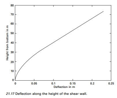
If the same problem has to be carried out by finite element packages, the coupled shear wall has to be modelled into four-node finite elements. Wilson (2002) recommends that four-node element cannot model linear bending if fine mesh is used and produces infinite stresses. Hence the coupled shear wall has to be modelled into beam, column and rigid zones, otherwise the results are not reliable. Parametric studies for the coupled shear considered could be easily made by changing α, ψ in symbolic programming whereas it cannot be done so easily with the finite element method. The deflected shape of the shear wall is shown in Fig. 21.17.