Applied Statistics - Summary | 12th Business Maths and Statistics : Chapter 9 : Applied Statistics
Chapter: 12th Business Maths and Statistics : Chapter 9 : Applied Statistics
Summary
Summary
In this chapter we have acquired the
knowledge of
Method
of Moving Averages
Three year moving averages: 
Four year moving averages: 
Method
of Least Squares
The straight line equation, Y = a + bX
Two Normal Equations, ΣY = n a + b ΣX ; ΣXY
= a ΣX + b ΣX2
Methods
of measuring Seasonal Variations-Method of Simple Averages:
Seasonal Index (S.I) = Seasonal Average/
Grand average X100
If
the data is given in months
S.I for Jan = Monthly Average ( for Jan)/
Grand average x 100
If
the data is given in quarter
S.I for Kth Quarter = Average of Kth
quarter/Grand average X 100
Continuous
distribution function
If X is a continuous random variable
with the probability density function f
X (x), then the function FX (x) is defined by
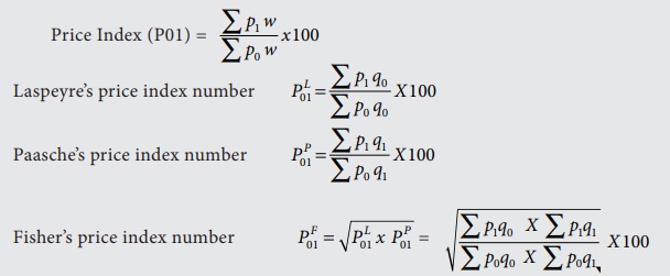
Weighted
Index Number
Price Index (P01), Laspeyre’s price index number, Paasche’s price index number, Fisher’s price index number

Time
Reversal Test :

Cost
of Living Index Number
Aggregate Expenditure Method = 
Family Budget Method = ∑ PV / ∑ V
Causes
of Variation
1. Chance Causes (or) Random causes 2.
Assignable Causes
Control
Charts
(i) Centre Line (CL) indicates the
desired standard level of the process.
(ii) Upper Control Limit (UCL) indicates
the upper limit of tolerance.
(iii) Lower Control Limit (LCL)
indicates the lower limit of tolerance.
(i) Centre Line (CL) indicates the
desired standard level of the process.
(ii) Upper Control Limit (UCL) indicates
the upper limit of tolerance.
(iii) Lower Control Limit (LCL)
indicates the lower limit of tolerance.
The control limits for ![]() chart
in two different cases are
chart
in two different cases are

The control limits for R chart in two
different cases are

Related Topics