Measurements of Trends: Method of Least Squares

Method of Least Squares

The line of best fit is a line from which the sum of the deviations of various points is zero. This is the best method for obtaining the trend values. It gives a convenient basis for calculating the line of best fit for the time series. It is a mathematical method for measuring trend. Further the sum of the squares of these deviations would be least when compared with other fitting methods. So, this method is known as the Method of Least Squares and satisfies the following conditions:

(i) The sum of the deviations of the actual values of Y and Ŷ (estimated value of Y) is Zero. that is Σ(Y–Ŷ) = 0.

(ii) The sum of squares of the deviations of the actual values of Y and Ŷ (estimated value of Y) is least. that is Σ(Y–Ŷ)2 is least ;

Procedure:

(i)  The straight line trend is represented by the equation Y = a + bX        …(1)

where  Y is the actual value, X is time, a, b are constants      

(ii)  The constants ‘a’ and ‘b’ are estimated by solving the following two normal

Equations   ΣY = n a + b ΣX   ...(2)

ΣXY = a ΣX + b ΣX2     ...(3)

Where ‘n’ = number of years given in the data.  

(iii) By taking the mid-point of the time as the origin, we get ΣX = 0

(iv) When ΣX = 0 , the two normal equations reduces to

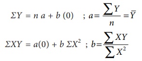
The constant ‘a’ gives the mean of Y and ‘b’ gives the rate of change (slope).

(v) By substituting the values of ‘a’ and ‘b’ in the trend equation (1), we get the Line of Best Fit.

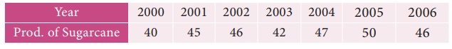
Example 9.6

Given below are the data relating to the production of sugarcane in a district.

Fit a straight line trend by the method of least squares and tabulate the trend values.

Solution:

Computation of trend values by the method of least squares (ODD Years).

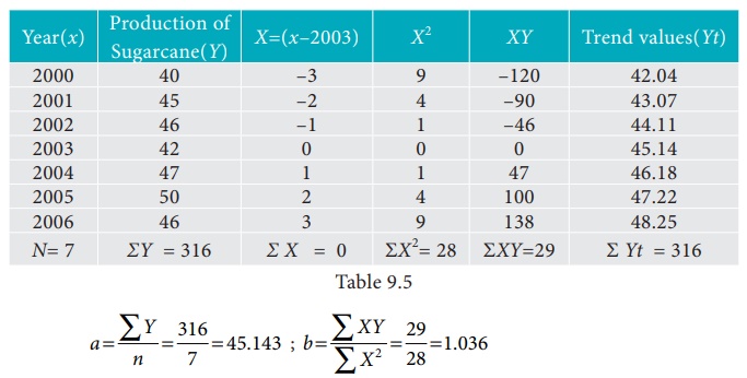
Therefore, the required equation of the straight line trend is given by

Y = a+bX;

Y = 45.143 + 1.036 (x-2003)

The trend values can be obtained by

When X = 2000 , Yt = 45.143 + 1.036(2000–2003) = 42.035

When X = 2001, Yt = 45.143 + 1.036(2001–2003) = 43.071,

similarly other values can be obtained.

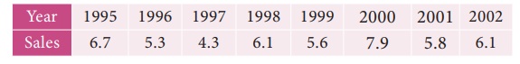
Example 9.7

Given below are the data relating to the sales of a product in a district.

Fit a straight line trend by the method of least squares and tabulate the trend values.

Solution:

Computation of trend values by the method of least squares.

In case of EVEN number of years, let us consider

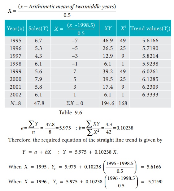
similarly other values can be obtained.

Note

(i) Future forecasts made by this method are based only on trend values.

(ii) The predicted values are more reliable in this method than the other methods.