Measurements of Trends

Measurements of Trends

Following are the methods by which we can measure the trend.

(i) Freehand or Graphic Method.

(ii) Method of Semi-Averages.

(iii) Method of Moving Averages.

(iv) Method of Least Squares.

(i) Freehand or Graphic Method.

It is the simplest and most flexible method for estimating a trend. We will see the working procedure of this method.

Procedure:

(a) Plot the time series data on a graph.

(b) Draw a freehand smooth curve joining the plotted points.

(c) Examine the direction of the trend based on the plotted points.

(d) Draw a straight line which will pass through the maximum number of plotted points.

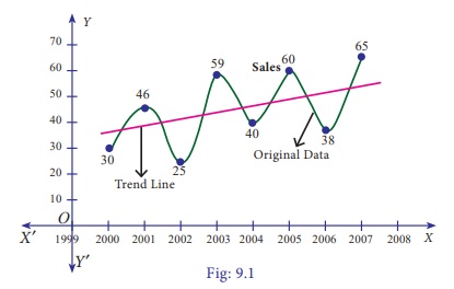
Example 9.1

Fit a trend line by the method of freehand method for the given data.

Solution:

Note

The trend drawn by the freehand method can be extended to predict the future values of the given data. However, this method is subjective in nature, predictions obtained by this method depends on the personal bias and judgement of the investigator handling the data.

(ii) Method of Semi-Averages

In this method, the semi-averages are calculated to find out the trend values. Now, we will see the working procedure of this method.

Procedure:

(i) The data is divided into two equal parts. In case of odd number of data, two equal parts can be made simply by omitting the middle year.

(ii) The average of each part is calculated, thus we get two points.

(iii) Each point is plotted at the mid-point (year) of each half.

(iv) Join the two points by a straight line.

(v) The straight line can be extended on either side.

(vi) This line is the trend line by the methods of semi-averages.

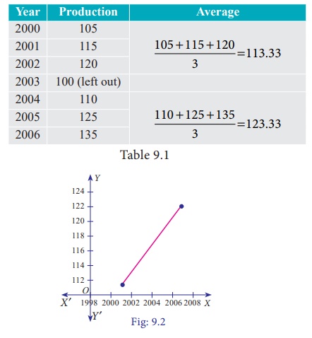
Example 9.2

Fit a trend line by the method of semi-averages for the given data.

Solution:

Since the number of years is odd(seven), we will leave the middle year’s production value and obtain the averages of first three years and last three years.

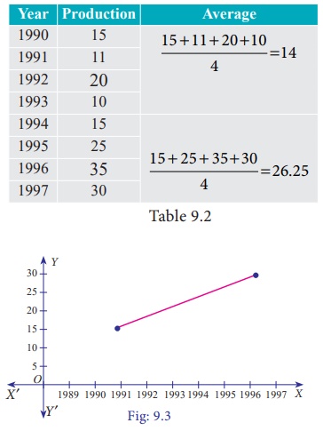
Example 9.3

Fit a trend line by the method of semi-averages for the given data.

Solution:

Since the number of years is even(eight), we can equally divide the given data it two equal parts and obtain the averages of first four years and last four years.

Note

(i) The future values can be predicted.

(ii) The trend values obtained by this method and the predicted values are not precise.

(iii) Method of Moving Averages

Moving Averages Method gives a trend with a fair degree of accuracy. In this method, we take arithmetic mean of the values for a certain time span. The time span can be three-years, four -years, five- years and so on depending on the data set and our interest. We will see the working procedure of this method.

Procedure:

(i) Decide the period of moving averages (three- years, four -years).

(ii) In case of odd years, averages can be obtained by calculating,

(iii) If the moving average is an odd number, there is no problem of centering it, the average value will be centered besides the second year for every three years.

(iv) In case of even years, averages can be obtained by calculating,

(v) If the moving average is an even number, the average of first four values will  be placed between 2 ^nd and 3^rd year, similarly the average of the second four values will be placed between 3^rd and 4^th year. These two averages will be again averaged and placed in the 3^rd year. This continues for rest of the values in the problem. This process is called as centering of the averages.

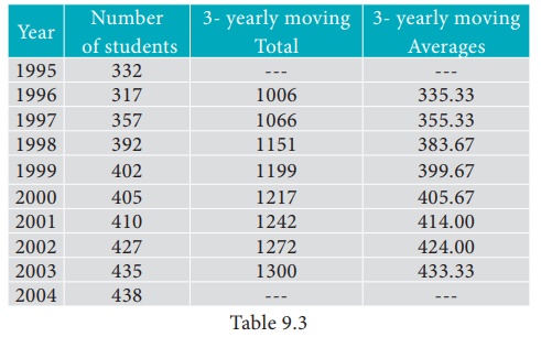
Example 9.4

Calculate three-yearly moving averages of number of students studying in a higher secondary school in a particular village from the following data.

Solution:

Computation of three- yearly moving averages.

Example 9.5

Calculate four-yearly moving averages of number of students studying in a higher secondary school in a particular city from the following data.

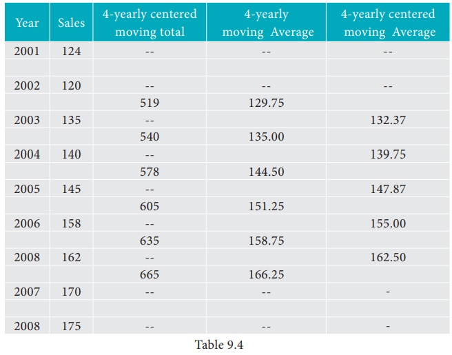
Solution:

Computation of four- yearly moving averages.

Note

The calculated 4-yearly centered moving average belongs to the particular year present in that row eg; 132.37 belongs to the year 2003.

(iv) Method of Least Squares

The line of best fit is a line from which the sum of the deviations of various points is zero. This is the best method for obtaining the trend values. It gives a convenient basis for calculating the line of best fit for the time series. It is a mathematical method for measuring trend. Further the sum of the squares of these deviations would be least when compared with other fitting methods. So, this method is known as the Method of Least Squares and satisfies the following conditions:

(i) The sum of the deviations of the actual values of Y and Ŷ (estimated value of Y) is Zero. that is Σ(Y–Ŷ) = 0.

(ii) The sum of squares of the deviations of the actual values of Y and Ŷ (estimated value of Y) is least. that is Σ(Y–Ŷ)² is least ;

Procedure:

(i)  The straight line trend is represented by the equation Y = a + bX        …(1)

where  Y is the actual value, X is time, a, b are constants      

(ii)  The constants ‘a’ and ‘b’ are estimated by solving the following two normal

Equations   ΣY = n a + b ΣX   ...(2)

ΣXY = a ΣX + b ΣX²     ...(3)

Where ‘n’ = number of years given in the data.  

(iii) By taking the mid-point of the time as the origin, we get ΣX = 0

(iv) When ΣX = 0 , the two normal equations reduces to

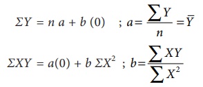
The constant ‘a’ gives the mean of Y and ‘b’ gives the rate of change (slope).

(v) By substituting the values of ‘a’ and ‘b’ in the trend equation (1), we get the Line of Best Fit.

Example 9.6

Given below are the data relating to the production of sugarcane in a district.

Fit a straight line trend by the method of least squares and tabulate the trend values.

Solution:

Computation of trend values by the method of least squares (ODD Years).

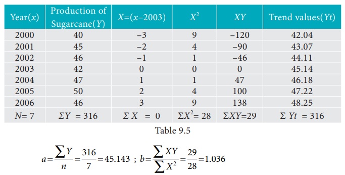
Therefore, the required equation of the straight line trend is given by

Y = a+bX;

Y = 45.143 + 1.036 (x-2003)

The trend values can be obtained by

When X = 2000 , Yt = 45.143 + 1.036(2000–2003) = 42.035

When X = 2001, Yt = 45.143 + 1.036(2001–2003) = 43.071,

similarly other values can be obtained.

Example 9.7

Given below are the data relating to the sales of a product in a district.

Fit a straight line trend by the method of least squares and tabulate the trend values.

Solution:

Computation of trend values by the method of least squares.

In case of EVEN number of years, let us consider

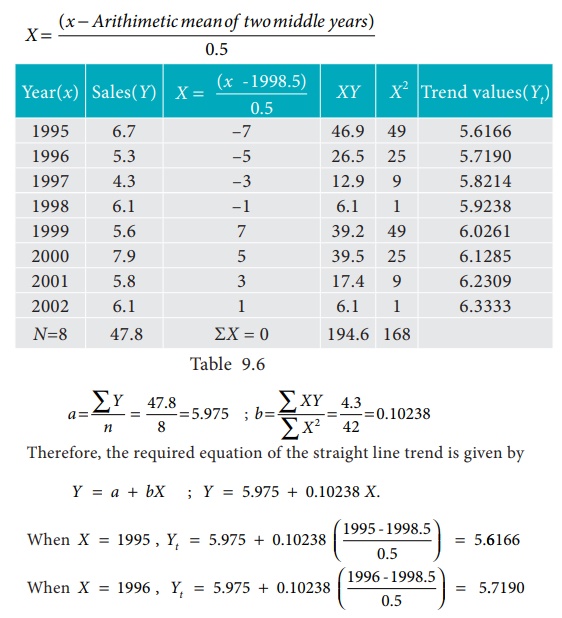
similarly other values can be obtained.

Note

(i) Future forecasts made by this method are based only on trend values.

(ii) The predicted values are more reliable in this method than the other methods.

(v) Methods of measuring Seasonal Variations By Simple Averages :

Seasonal Variations can be measured by the method of simple average. The data should be available in season wise likely weeks, months, quarters.

Method of Simple Averages:

This is the simplest and easiest method for studying Seasonal Variations. The procedure of simple average method is outlined below.

Procedure:

(i) Arrange the data by months, quarters or years according to the data given.

(ii) Find the sum of the each months, quarters or year.

(iii) Find the average of each months, quarters or year.

(iv) Find the average of averages, and it is called Grand Average (G)

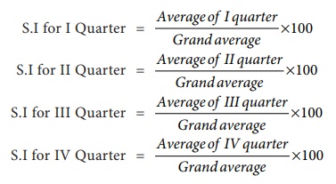
(v) Compute Seasonal Index for every season (i.e) months, quarters or year is given by

(vi) If the data is given in months

Similarly we can calculate SI for all other months.

(vii) If the data is given in quarter

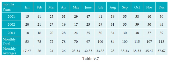
Example 9.8

Calculate the seasonal index for the monthly sales of a product using the method of simple averages.

Solution:

Computation of seasonal Indices by method of simple averages.

Similarly other seasonal index values can be obtained.

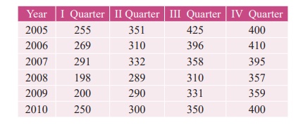
Example 9.9

Calculate the seasonal index for the quarterly production of a product using the method of simple averages.

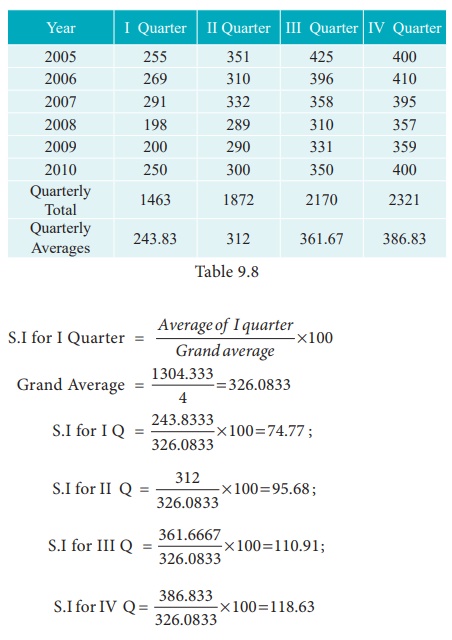
Solution:

Computation of Seasonal Index by the method of simple averages.