Inelastic response spectra

Inelastic response spectra

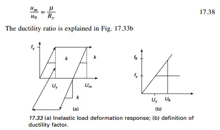
While the foregoing discussion has been for elastic response spectra, most structures are not expected or even designed to remain elastic under strong ground motions. Rather, structures are expected to enter the inelastic region, and the extent to which they behave inelastically can be defined by the ductility factor

assuming the simplest force deformation relationship is chosen. Figure 17.33a shows the elastic perfectly plastic (elasto-plastic) force deformation relation, f _s (u , sign u˙). The elastic stiffness is K and the post-yield stiffness is zero. The yield strength is f_y and the yield deflection is u_y. During unloading the algebraic sign of u˙ is negative and during reloading the algebraic sign of u˙ is positive and hence the hysteretic system occurs along a path parallel to the initial elastic branch without any deterioration of stiffness and strength. Within the linear elastic range the natural vibration period is T_n (T_n = 2π/ω_n) and the damping ratio is ρ.

1Ductility factor and yield strength reduction factor

The yield strength reduction factor R_y is defined as

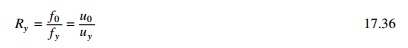
where f₀ and u₀ are the minimum yield strength and yield deflection required for the structure to remain elastic during ground motion.

ductility factor = u_m/u_{y             --- ----} 17.37

The inelastic deformation ratio is defined as the ratio of deflection of inelastic and the corresponding linear system related by µ and R_y.

2Equations of motion and controlled parameters

The governing equation of motion is

The same numerical procedures discussed in Chapter 7 can also be applied here with the difference that the time instants must be detected accurately enough when the system changes from elastic to yield branch.

For a given ground excitation u˙˙g (t ) , u(t) depends on three system parameters ωn(Tn = 2π/ωn), ρ, and uy and the ductility factor µ depends on  ω_nρ and R_y

3Inelastic response shock spectrum

Peak deformation and ductility demand

The deformation response of an inelastic system is obtained from its initial elastic vibration period T_n and damping factor ρ and force deflection relation and its corresponding linear system are also obtained.

Inelastic response spectra can be calculated in the time domain by direct integration, analogous to elastic response spectra but with structural stiffness as a nonlinear function of displacements K = K(u). If elastic plastic behaviour is assumed, then elastic response spectra on the basis that at high periods T_n > 33 s (f_n < 0.03 Hz) displacements are the same and at high frequencies and at low periods T_n < 1/33 s (f_n > 33 Hz) acceleration are equal and at intermediate periods (frequencies) the absorbed energy is preserved.

An inelastic design spectrum is most commonly created directly from the elastic design spectrum. Observe then the spectral velocity S_v, spectral displacement S_d, converted to force-based design values by dividing them by the ductility factor:

In the acceleration constant region, the reduction factor R_y is attained by equating elastic and inelastic strain energies. The resultant reduction factor is 2 µ  RooT(− 1) . The inelastic design spectrum follows elastic spectrum in the acceleration constant region where it is multiplied by µ / 2 µ RooT(− 1) . This quantification of relative displacement maxima is usually referred to as ‘equal displacement’ when incorporated with the description of the design process.

Several researchers have proposed equations of variation of R_y with T_n, and µ. The elastic spectrum equation for R_y goes back to the work of Velestos and Newmark:

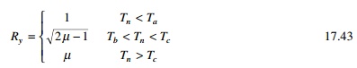
where the periods T_a, T_b,…, T_f separating the spectral regions are already defined. The basis of the well-known design spectra developed by Newmark and Hall is plotted for several values of µ in log–log format as shown in Fig. 17.34, where sloping straight lines are included to provide transition among the three constant segments. The construction of inelastic design spectrum is shown in Fig. 17.35. The inelastic design spectrum for 5% damping 84%

u˙˙_g  = 1g ; u˙_g  = 122 cm/s, u_g0 = 91.44 cm is shown in logarithmic and normal scale in Figs 17.36 and 17.37 respectively.

Spectra such as those described above provides the basis for safety evaluation of new and existing structures which will be discussed in later chapters.