Chapter: Analysis and Design of Algorithm
Fundamentals of the Analysis of Algorithm Efficiency
FUNDAMENTALS OF THE ANALYSIS OF
ALGORITHM EFFICIENCY
Fundamentals
of Analysis of Algorithm:
1
Analysis of Framework
2
Measuring an input size
3 Units
for measuring runtime
4 Worst
case, Best case and Average case
5
Asymptotic Notations
1 ANALYSIS FRAME WORK
ŌÖ” there
are two kinds of efficiency
ŌÖ” Time
efficiency - indicates how fast an algorithm in question runs.
ŌÖ” Space
efficiency - deals with the extra space the algorithm requires.
2 MEASURING AN INPUT SIZE
ŌÖ”
An algorithm's efficiency as a function of some
parameter n indicating the algorithm's input size.
ŌÖ”
In most cases, selecting such a parameter is quite
straightforward.
ŌÖ”
For example, it will be the size of the list for
problems of sorting, searching, finding the list's smallest element, and most
other problems dealing with lists.
ŌÖ”
For the problem of evaluating a polynomial p(x) = a n x n+ . . . + a 0 of degree n, it will be
the polynomial's degree or the number of its coefficients, which is larger by
one than its degree.
ŌÖ”
There are situations, of course, where the choice
of a parameter indicating an input size does matter.
ŌÖ” Example - computing the product of two
n-by-n matrices.
ŌÖ” There are
two natural measures of size for this problem.
ŌÖ”
The matrix order n.
ŌÖ”
The total number of elements N in the matrices being
multiplied.
ŌÖ”
Since there is a simple formula relating these two
measures, we can easily switch from one to the other, but the answer about an
algorithm's efficiency will be qualitatively different depending on which of
the two measures we use.
ŌÖ”
The choice of an appropriate size metric can be
influenced by operations of the algorithm in question. For example, how should
we measure an input's size for a spell-checking algorithm? If the algorithm
examines individual characters of its input, then we should measure the size by
the number of characters; if it works by processing words, we should count
their number in the input.
ŌÖ”
We should make a special note about measuring size
of inputs for algorithms involving properties of numbers (e.g., checking
whether a given integer n is prime).
ŌÖ”
For such algorithms, computer scientists prefer
measuring size by the number b of bits in the n's binary representation:
b=|log2n|+1
![]()
ŌÖ”
This metric usually gives a better idea about
efficiency of algorithms in question.
3 UNITS FOR MEASURING RUN TIME:
ŌÖ”
We can simply use some standard unit of time
measurement-a second, a millisecond, and so on-to measure the running time of a
program implementing the algorithm.
ŌÖ”
There are obvious drawbacks to such an approach.
They are
ŌÖ”
Dependence on the speed of a particular computer
ŌÖ”
Dependence on the quality of a program implementing
the algorithm
ŌÖ”
The compiler used in generating the machine code
ŌÖ”
The difficulty of clocking the actual running time
of the program.
ŌÖ”
Since we are in need to measure algorithm
efficiency, we should have a metric that does not depend on these extraneous
factors.
ŌÖ”
One possible approach is to count the number of
times each of the algorithm's operations is executed. This approach is both
difficult and unnecessary.
ŌÖ”
The main objective is to identify the most
important operation of the algorithm, called
the basic
operation, the operation contributing the most to the total running time, and
compute the number of times the basic operation is executed.
4 WORST CASE, BEST CASE AND
AVERAGE CASE EFFICIENCES
ŌÖ”
It is reasonable to measure an algorithm's
efficiency as a function of a parameter indicating the size of the algorithm's
input.
ŌÖ”
But there are many algorithms for which running
time depends not only on an input size but also on the specifics of a
particular input.
ŌÖ”
Example,
sequential search. This is a straightforward algorithm that searches
for a given item (some search key K)
in a list of n elements by checking successive elements of the list until
either a match with the search key is found or the list is exhausted.
ŌÖ”
Here is the algorithm's pseudo code, in which, for
simplicity, a list is implemented as an array. (It also assumes that the second
condition A[i] i= K will not be checked if the first one, which checks that the
array's index does not exceed its upper bound, fails.)
ALGORITHM Sequential
Search(A[0..n -1], K)
//Searches for a given value in a given array by
sequential search //Input: An array A[0..n -1] and a search key K
//Output: Returns the index of the first element of
A that matches K // or -1 ifthere are no matching elements
iŌåÉ0
while i < n
and A[i] ŌēĀ K do
iŌåÉi+1
if i < n return i else return -1
ŌÖ”
Clearly, the running time of this algorithm can be
quite different for the same list size n.
Worst case efficiency
ŌÖ”
The worst-case efficiency of an algorithm is its
efficiency for the worst-case input of size n, which is an input (or inputs) of
size n for which the algorithm runs the longest among all possible inputs of
that size.
ŌÖ”
In the worst case, when there are no matching
elements or the first matching element happens to be the last one on the list,
the algorithm makes the largest number of key comparisons among all possible
inputs of size n:
Cworst (n) = n.
ŌÖ”
The way to determine is quite straightforward
ŌÖ”
To analyze the algorithm to see what kind of inputs
yield the largest value of the basic operation's count C(n) among all possible
inputs of size n and then compute this worst-case value C worst (n)
ŌÖ”
The worst-case analysis provides very important
information about an algorithm's efficiency by bounding its running time from
above. In other words, it guarantees that for any instance of size n, the
running time will not exceed C worst (n) its running time on the worst-case inputs.
Best case Efficiency
ŌÖ”
The best-case efficiency of an algorithm is its
efficiency for the best-case input of size n, which is an input (or inputs) of
size n for which the algorithm runs the fastest among all possible inputs of
that size.
ŌÖ”
We can analyze the best case efficiency as follows.
ŌÖ”
First, determine the kind of inputs for which the
count C (n) will be the smallest among all possible inputs of size n. (Note
that the best case does not mean the smallest input; it means the input of size
n for which the algorithm runs the fastest.)
ŌÖ”
Then ascertain the value of C (n) on these most
convenient inputs.
ŌÖ”
Example- for sequential search, best-case inputs
will be lists of size n with their first elements equal to a search key;
accordingly, Cbest(n) = 1.
ŌÖ”
The analysis of the best-case efficiency is not
nearly as important as that of the worst-case efficiency.
ŌÖ”
But it is not completely useless. For example,
there is a sorting algorithm (insertion sort) for which the best-case inputs
are already sorted arrays on which the algorithm works very fast.
ŌÖ”
Thus, such an algorithm might well be the method of
choice for applications dealing with almost sorted arrays. And, of course, if
the best-case efficiency of an algorithm is unsatisfactory, we can immediately
discard it without further analysis.
Average case efficiency
ŌÖ”
It yields the information about an algorithm about
an algorithmŌĆśs behaviour on a ŌĆĢtypicalŌĆ¢ and ŌĆĢrandomŌĆ¢ input.
ŌÖ”
To analyze the algorithm's average-case efficiency,
we must make some assumptions about possible inputs of size n.
ŌÖ”
The investigation of the average case efficiency is
considerably more difficult than investigation of the worst case and best case
efficiency.
ŌÖ”
It involves dividing all instances of size n .into
several classes so that for each instance of the class the number of times the
algorithm's basic operation is executed is the same.
ŌÖ”
Then a probability distribution of inputs needs to
be obtained or assumed so that the expected value of the basic operation's
count can then be derived.
The
average number of key comparisions Cavg(n) can be computed as
follows,
ŌÖ”
let us consider again sequential search. The
standard assumptions are,
ŌÖ”
In the case of a successful search, the probability
of the first match occurring in the ith position of the list is pin for every
i, and the number of comparisons made by the algorithm in such a situation is
obviously i.
ŌÖ”
In the case of an unsuccessful search, the number
of comparisons is n with the probability of such a search being (1 - p).
Therefore,
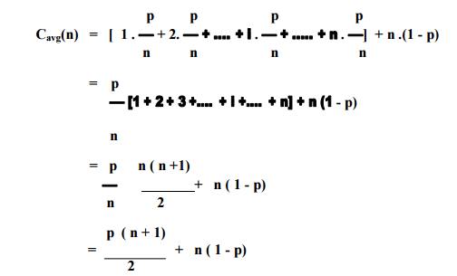
ŌÖ”
Example, if p = 1 (i.e., the search must be
successful), the average number of key comparisons made by sequential search is
(n + 1) /2.
ŌÖ”
If p = 0 (i.e., the search must be unsuccessful),
the average number of key comparisons will be n because the algorithm will
inspect all n elements on all such inputs.
5 Asymptotic Notations
Step
count is to compare time complexity of two programs that compute same function
and also to predict the growth in run time as instance characteristics changes.
Determining exact step count is difficult and not necessary also. Because the
values are not exact quantities. We need only comparative statements like c1n2
Ōēż tp(n) Ōēż c2n2.
For
example, consider two programs with complexities c1n2 + c2n
and c3n respectively. For small values of n, complexity depend upon
values of c1, c2 and c3. But there will also
be an n beyond which complexity of c3n is better than that of c1n2
+ c2n.This value of n is called break-even point. If this point is
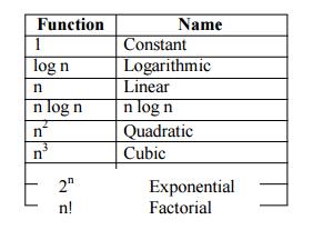
zero, c 3n is always faster (or at least as fast). Common asymptotic
functions are given below.
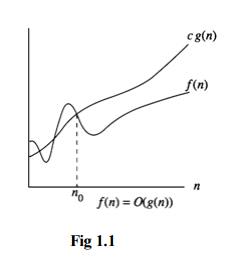
BigŌĆśOhŌĆÖNotation(O)
O(g(n)) =
{ f(n) : there exist positive constants c and n0 such that 0 Ōēż f(n)
Ōēż cg(n) for all n Ōēź
n0
}
It is the
upper bound of any function. Hence it denotes the worse case complexity of any
algorithm. We can represent it graphically as
Find the
Big ŌĆŚOhŌĆś for the following functions:
Linear Functions
Example 1.6 f(n) = 3n
+ 2
General
form is f(n) Ōēż cg(n)
When n Ōēź 2, 3n
+ 2 Ōēż 3n + n = 4n
Hence
f(n) = O(n), here c = 4 and n0 = 2
When n Ōēź 1, 3n
+ 2 Ōēż 3n + 2n = 5n
Hence
f(n) = O(n), here c = 5 and n0 = 1
Hence we
can have different c,n0 pairs satisfying for a given function.
Example f(n) = 3n
+ 3
When n Ōēź
3, 3n + 3 Ōēż 3n + n = 4n Hence f(n) = O(n), here c = 4 and n0 = 3
Example
f(n) =
100n + 6
When n Ōēź
6, 100n + 6 Ōēż 100n + n = 101n Hence f(n) = O(n), here c = 101 and n0
= 6
Quadratic Functions
Example 1.9
f(n) =
10n2 + 4n + 2
When n Ōēź 2, 10n2
+ 4n + 2 Ōēż 10n2 + 5n
When n Ōēź
5, 5n Ōēż n2, 10n2 + 4n + 2 Ōēż 10n2 + n2
= 11n2 Hence f(n) = O(n2), here c = 11 and n0
= 5
Example 1.10
f(n) =
1000n2 + 100n - 6
f(n) Ōēż
1000n2 + 100n for all values of n.
When n Ōēź
100, 5n Ōēż n2, f(n) Ōēż 1000n2 + n2 = 1001n2
Hence f(n) = O(n2), here c = 1001 and n0 = 100
Exponential Functions
Example 1.11 f(n) =
6*2n + n2
When n Ōēź 4, n2
Ōēż 2n
So f(n) Ōēż
6*2n + 2n = 7*2n
Hence
f(n) = O(2n), here c = 7 and n0 = 4
Constant Functions
Example 1.12 f(n) = 10
f(n) =
O(1), because f(n) Ōēż 10*1
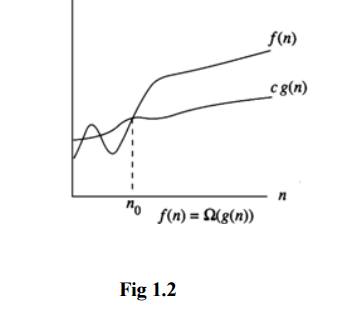
OmegaNotation(Ōä”)
Ōä” (g(n))
= { f(n) : there exist positive constants c and n0 such that 0 Ōēż
cg(n) Ōēż f(n) for all n
Ōēź n0
}
It is the
lower bound of any function. Hence it denotes the best case complexity of any
algorithm. We can represent it graphically as
Example 1.13 f(n) = 3n
+ 2
3n + 2
> 3n for all n. Hence f(n) = Ōä”(n)
Similarly
we can solve all the examples specified under Big ŌĆŚOhŌĆś.
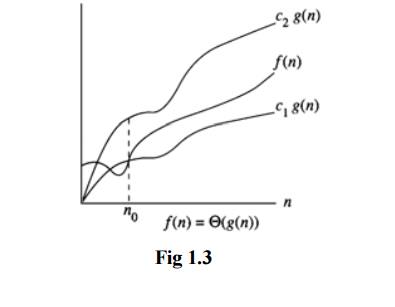
ThetaNotation(╬ś)
![]()
╬ś(g(n)) =
{f(n) : there exist positive constants c1,c2 and n0
such that c1g(n) Ōēżf(n) Ōēżc2g(n) for all n Ōēź n0
}
If f(n) =
╬ś(g(n)), all values of n right to n0 f(n) lies on or above c1g(n)
and on or below c2g(n). Hence it is asymptotic tight bound for f(n).
Little-O Notation
For
non-negative functions, f(n) and g(n), f(n) is little o of g(n) if and only if
f(n) = O(g(n)), but f(n) ŌēĀ ╬ś(g(n)). This is denoted as "f(n) =
o(g(n))".
This
represents a loose bounding version of Big O. g(n) bounds from the top, but it
does not bound the bottom.
Little Omega Notation
For
non-negative functions, f(n) and g(n), f(n) is little omega of g(n) if and only
if f(n) = ╬®(g(n)), but f(n) ŌēĀ ╬ś(g(n)). This is denoted as "f(n) =
Žē(g(n))".
Much like
Little Oh, this is the equivalent for Big Omega. g(n) is a loose lower boundary
of the function f(n); it bounds from the bottom, but not from the top.
Conditional asymptotic notation
Many algorithms are easier to analyse if initially
we restrict our attention to instances whose size satisfies a certain
condition, such as being a power of 2. Consider, for example, the divide and
conquer algorithm for multiplying large integers that we saw in the
Introduction. Let n be the size of
the integers to be multiplied.
The algorithm proceeds directly if n = 1, which requires a microseconds for an appropriate
constant a. If n>1, the algorithm proceeds by multiplying four pairs of
integers of size ![]() three if we use the better algorithm).
Moreover, it takes a linear amount of time to carry out additional tasks. For
simplicity, let us say that the additional work takes at most bn microseconds for an appropriate
constant b.
three if we use the better algorithm).
Moreover, it takes a linear amount of time to carry out additional tasks. For
simplicity, let us say that the additional work takes at most bn microseconds for an appropriate
constant b.
![]()
Properties of Big-Oh Notation
Generally,
we use asymptotic notation as a convenient way to examine what can happen in a
function in the worst case or in the best case. For example, if you want to
write a function that searches through an array of numbers and returns the
smallest one:
function
find-min(array a[1..n]) let j :=
for i := 1 to n:
j :=
min(j, a[i] ) repeat
return j end
Regardless
of how big or small the array is, every time we run find-min, we have to
initialize the i and j integer variables and return j at the end. Therefore, we
can just think of those parts of the function as constant and ignore them.
So, how
can we use asymptotic notation to discuss the find-min function? If we search
through an array with 87 elements, then the for loop iterates 87 times, even if
the very first element we hit turns out to be the minimum. Likewise, for n elements,
the for loop iterates n times. Therefore we say the function runs in time O(n).
function find-min-plus-max(array
a[1..n] )
// First, find the smallest element in the array let j
:= ;
for i := 1 to n:
j :=
min(j, a[i] ) repeat
let minim := j
// Now, find the biggest element, add it to the
smallest and j := ;
for i := 1 to n:
j :=
max(j, a[i] ) repeat
let maxim := j
// return the sum of the two
return minim + maxim;
end
What's the running time for find-min-plus-max?
There are two for loops, that each iterate n times, so the running time is
clearly O(2n). Because 2 is a constant, we throw it away and write the running
time as O(n). Why can you do this? If you recall the definition of Big-O
notation, the function whose bound you're testing can be multiplied by some
constant. If f(x)=2x, we can see that if g(x) = x, then the Big-O condition
holds. Thus O(2n) = O(n). This rule is general for the various asymptotic
notations.
Recurrence
When an
algorithm contains a recursive call to itself, its running time can often be
described by a recurrence
Recurrence Equation
A
recurrence relation is an equation that recursively defines a sequence. Each
term of the sequence is defined as a function of the preceding terms. A
difference equation is a specific type of recurrence relation.
An
example of a recurrence relation is the logistic map:
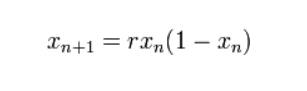
Related Topics