Algorithm: Branch and Bound

BRANCH-AND-BOUND

Backtracking is to cut off a branch of the problem‘s state-space tree as soon as we can deduce that it cannot lead to a solution.

This idea can be strengthened further if we deal with an optimization problem, one that seeks to minimize or maximize an objective function, usually subject to some constraints. Note that in the standard terminology of optimization problems, a feasible solution is a point in the problem‘s search space that satisfies all the problem‘s constraints

(e.g. a Hamiltonian circuit in the traveling salesman problem, a subset of items whose total weight does not exceed the knapsack‘s capacity), while an optimal solution is a feasible solution with the best value of the objective function (e.g., the shortest Hamiltonian circuit, the most valuable subset of items that fit the knapsack).

Compared to backtracking, branch-and-bound requires two additional items.

A way to provide, for every node of a state-space tree, a bound on the best value of the objective functions on any solution that can be obtained by adding further components to the partial solution represented by the node

The value of the best solution seen so far

GENERAL METHOD

If this information is available, we can compare a node‘s bound value with the value of the best solution seen so far:

if the bound value is not better than the best solution seen so far—i.e., not smaller for a minimization problem and not larger for a maximization problem—the node is nonpromising and can be terminated (some people say the branch is pruned) because no solution obtained from it can yield a better solution than the one already available.

E.g. Termination of search path

In general, we terminate a search path at the current node in a state-space tree of a branch-and-bound algorithm for any one of the following three reasons:

1.     The value of the node‘s bound is not better than the value of the best solution seen so far.

2.     The node represents no feasible solutions because the constraints of the problem are already violated.

3.     The subset of feasible solutions represented by the node consists of a single point (and hence no further choices can be made)—in this case we compare the value of the objective function for this feasible solution with that of the best solution seen so far and update the latter with the former if the new solution is better.

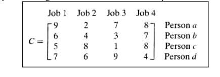
 ASSIGNMENT PROBLEM

Let us illustrate the branch-and-bound approach by applying it to the problem of assigning n people to n jobs. So that the total cost of the assignment is as small as possible.

An instance of the assignment problem is specified by an n-by-n cost matrix C so that we can state the problem as follows:

Select one element in each row of the matrix so that no two selected elements are in the same column and their sum is the smallest possible.

Demonstrate of solving this problem using the branch-and-bound

This is done by considering the same small instance of the problem:

To find a lower bound on the cost of an optimal selection without actually solving the problem, we can do several methods.

For example, it is clear that the cost of any solution, including an optimal one, cannot be

smaller than the sum of the smallest elements in each of the matrix‘s rows. For the instance here, this sum is 2 +3 + 1 + 4 = 10.

It is important to stress that this is not the cost of any legitimate selection (3 and 1 came from the same column of the matrix); it is just a lower bound on the cost of any legitimate selection.

We Can and will apply the same thinking to partially constructed solutions. For example, for any legitimate selection that selects 9 from the first row, the lower bound will be 9 + 3 + 1 + 4 = 17.

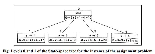
Fig: Levels 0 and 1 of the State-space tree for the instance of the assignment problem

(being solved with the best-first branch-and- bound algorithm. The number above a node shows the order in which the node was generated. A node‘s fields indicate the job number assigned to person a, and the lower bound value, lb for this node.)

This problem deals with the order in which the tree‘s nodes will he generated. Rather than generating a single child of the last promising node as we did in backtracking, we wilt generate all the children of the most promising node among non-terminated leaves in the current tree. (Non-terminated, je., still promising, leaves are also called live.)

To find which of the nodes is most promising, we are comparing the lower bounds of the live node. It is sensible to consider a node with the best bound as most promising, although this does not, of course, preclude the possibility that an optimal solution will ultimately belong to a different branch of the state-space tree.

This variation of the strategy is called the best-first branch-and-bound. Returning to the instance of the assignment problem given earlier, we start with the root that corresponds to no elements selected from the cost matrix. As the lower bound value for the root, denoted lb is 10.

The nodes on the first level of the free correspond to four elements (jobs) in the first row of the matrix since they are each a potential selection for the first component of the solution. So we have four live leaves (nodes 1 through 4) that may contain an optimal solution. The most promising of them is node 2 because it has the smallest lower bound value.

Following our best-first search strategy, we branch out from that node first by considering the three different ways of selecting an element from the second row and not in the second column—the three different jobs that can be assigned to person b.

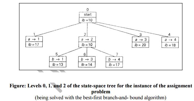
Figure: Levels 0, 1. and 2 of the state-space tree for the instance of the assignment problem

(being solved with the best-first branch-and- bound algorithm)

Of the six live leaves (nodes 1, 3, 4, 5, 6, and 7) that may contain an optimal solution, we again choose the one with the smallest lower bound, node 5.

First, we consider selecting the third column‘s element from c‘s row (i.e., assigning person c to job 3); this leaves us with no choice but to select the element from the fourth column of d‘s row (assigning person d to job 4).

This yields leafs that corresponds to the feasible solution (a →2, b→1, c→3, d →4) with (he total cost of 13. Its sibling, node 9, corresponds to the feasible solution {a → 2, b →1, c

→ 4, d → 3) with the total cost of 25, Since its cost is larger than the cost of the solution represented by leafs, node 9 is simply terminated.

Note that if its cost were smaller than 13. we would have to replace the information about the best solution seen so far with the data provided by this node.

Now, as we inspect each of the live leaves of the last state-space tree (nodes 1, 3, 4, 6, and

7 in the following figure), we discover that their lower bound values are not smaller than 13 the value of the best selection seen so far (leaf 8).

Hence we terminate all of them and recognize the solution represented by leaf 8 as the optima) solution to the problem.

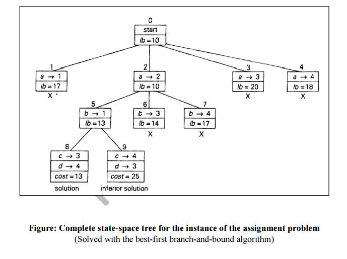
Figure: Complete state-space tree for the instance of the assignment problem

(Solved with the best-first branch-and-bound algorithm)

KNAPSACK PROBLEM

Illustration

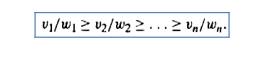
Given n items of known weights w_i and values v_i, i = 1,2,..., n, and a knapsack of capacity W, find the most valuable subset of the items that fit in the knapsack. It is convenient to order the items of a given instance in descending order by their value-to-weight ratios. Then the first item gives the best payoff per weight unit and the last one gives the worst payoff per weight unit, with ties resolved arbitrarily:

It is natural to structure the state-space tree for this problem as a binary tree constructed as follows (following figure).

Each node on the ith level of this tree, 0 ≤ i ≤ n, represents all the subsets of n items that include a particular selection made from the first i ordered items. This particular selection is uniquely determined by a path from the root to the node: a branch going to the left indicates the inclusion of the next item while the branch going to the right indicates its exclusion.

We record the total weight w and the total value v of this selection in the node, along with some upper bound ub on the value of any subset that can be obtained by adding zero or more items to this selection.

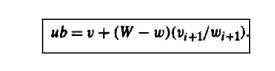
A simple way to compute the upper bound ub is to add to v, the total value of the items already selected, the product of the remaining capacity of the knapsack W - w and the best per unit payoff among the remaining items, which is v_i+1/w_i+1 :

As a specific example, let us apply the branch-and-bound algorithm to die same instance of

the knapsack problem , At the root of the state-space tree (in the following figure), no items have been selected as yet. Hence, both the total weight of the items already selected w and their total value v are equal to 0.

The value of the upper bound computed by formula (ub=v+(W-w)(v_i+1/w_i+1) is $100. Node 1, the left child of the root, represents the subsets that include item, 1.

The total weight and value of the items already included are 4 and $40, respectively; the value of the upper bound is 40 + (10-4)*6 = $76.

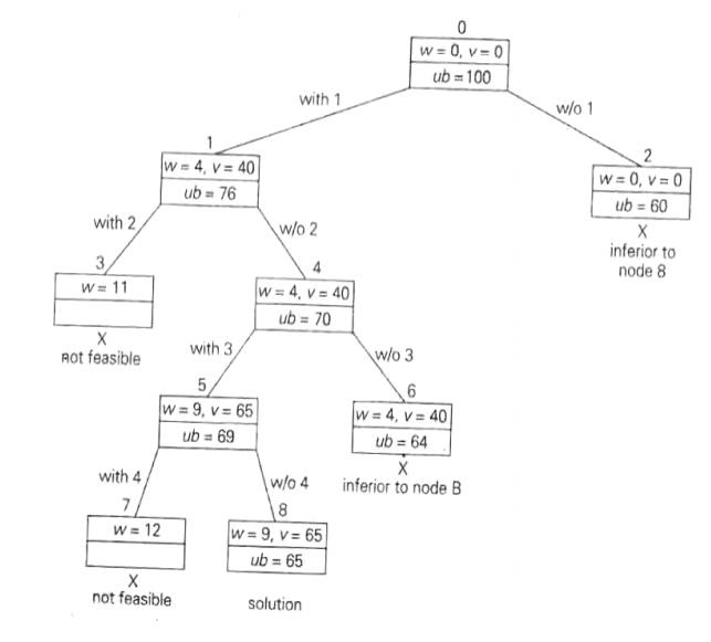
Fig: State-space tree of the branch-and-bound algorithm for the instance of the knapsack problem

Node 2 represents the subsets that do not include item 1. Accordingly, w = 0, v= $0, and ub=0+(10-0)*6=$60.

Since node 1 has a larger upper bound than the upper bound of node 2, it is more promising for this maximization problem, and we branch from node 1 first. Its children—nodes 3 and 4—represent subsets with item 1 and with and without item 2, respectively.

Since the total weight w of every subset represented by node 3 exceeds the knapsack‘s capacity, node 3 can be terminated immediately. Node 4 has the same values of w and u as its parent; the upper bound ub is equal to 40 + (10-4)*5 = $70.

Selecting node 4 over node 2 for the next branching, we get nodes 5 and 6 by respectively including and excluding item 3. The total weights and values as well as the upper bounds for these nodes are computed in the same way as for the preceding nodes.

Branching from node 5 yields node 7, represents no feasible solutions and node 8 that represents just a single subset {1, 3}.

The remaining live nodes 2 and 6 have smaller upper-bound values than the value of the solution represented by node 8. Hence, both can be terminated making the subset {1, 3} of node 8 the optimal solution to the problem.

Solving the knapsack problem by a branch-and-bound algorithm has a rather unusual characteristic.

Typically, internal nodes of a state-space tree do not define a point of the problem‘s search space, because some of the solution‘s components remain undefined. For the knapsack problem, however, every node of the tree represents a subset of the items given.

We can use this fact to update the information about the best subset seen so far after generating each new node in the tree. If we did this for the instance investigated above, we could have terminated nodes 2 & 6 before node 8 was generated because they both are inferior to the subset of value $65 of node 5.

INTRODUCTION TO NP-HARD AND NP-COMPLETENESS

P: the class of decision problems that are solvable in O(p(n)) time, where p(n) is a polynomial of problem‘s input size n

Examples:

b  searching

b element uniqueness b graph connectivity b graph acyclicity

primality testing (finally proved in 2002)

NP (nondeterministic polynomial): class of decision problems whose proposed solutions can be verified in polynomial time = solvable by a nondeterministic polynomial algorithm

A nondeterministic polynomial algorithm is an abstract two-stage procedure that: b generates a random string purported to solve the problem

b  checks whether this solution is correct in polynomial time

E.g. Problem: Is a boolean expression in its conjunctive normal form (CNF) satisfiable, i.e., are there values of its variables that makes it true?

This problem is in NP. Nondeterministic algorithm: b Guess truth assignment

b Substitute the values into the CNF formula to see if it evaluates to true Example: (A | ¬B | ¬C) & (A | B) & (¬B | ¬D | E) & (¬D | ¬E)

Truth assignments:

A B C D E 0 0 0 0 0

.  .  .

1 1 1 1 1

Checking phase: O(n)

1. PROBLEMS ARE IN NP?

b  Hamiltonian circuit existence

b       Partition problem: Is it possible to partition a set of n integers into two disjoint subsets with the same sum?

b       Decision versions of TSP, knapsack problem, graph coloring, and many other combinatorial optimization problems. (Few exceptions include: MST, shortest paths)

b       All the problems in P can also be solved in this manner (but no guessing is necessary), so we have:

 P inculde NP

b  Big question:  P = NP ?

NP problems

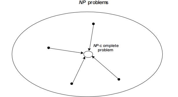
NP Hard problem:

–   Most problems discussed are efficient (poly time)

–   An interesting set of hard problems: NP-complete.

•         A decision problem D is NP-complete if it‘s as hard as any problem in NP, i.e.,  D is in NP

  every problem in NP is polynomial-time reducible to D

Cook’s theorem (1971): CNF-sat is NP-complete

Other NP-complete problems obtained through polynomial-time reductions from a known NP-complete problem

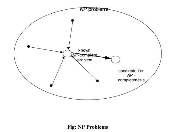
Fig: NP Problems

Examples:

TSP, knapsack, partition, graph-coloring and hundreds of other problems of combinatorial nature

v   P = NP would imply that every problem in NP, including all NP-complete problems, could be solved in polynomial time

v   If a polynomial-time algorithm for just one NP-complete problem is discovered,

then every problem in NP can be solved in polynomial time, i.e., P = NP

v        Most but not all researchers believe that P NP , i.e. P is a proper subset of NP