Greedy Method Algorithm

GREEDY TECHNIQUES

The greedy approach suggests constructing a solution through a sequence of steps, each expanding a partially constructed solution obtained so far, until a complete solution to the problem is reached. On each step—and this is the central point of this technique—the choice made must be

•       Feasible, i.e., it has to satisfy the problem‘s constraints.

•       Locally optimal, i.e., it has to be the best local choice among all feasible choices available on that step.

•       Irrevocable, i.e., once made, it cannot be changed on subsequent steps of the algorithm.

GENERAL METHOD

PRIM’S ALGORITHM

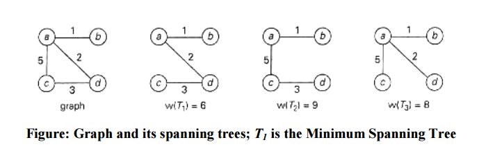
Definition:

A spanning tree of a connected graph is its connected acyclic subgraph (i.e., a tree) that contains all the vertices of the graph. A minimum spanning tree of a weighted connected graph is its spanning tree of the smallest weight, where the weight of a tree is defined as the sum of the weights on all its edges. The minimum spanning tree problem is the problem of finding a minimum spanning tree for a given weighted connected graph.

Two serious difficulties to construct Minimum Spanning Tree

1.     The number of spanning trees grows exponentially with the graph size (at least for dense graphs).

2.   Generating all spanning trees for a given graph is not easy.

Prim‘s algorithm constructs a minimum spanning tree through a sequence of expanding subtrees. The initial subtree in such a sequence consists of a single vertex selected arbitrarily from the set V of the graph‘s vertices. On each iteration, we expand the current tree in the greedy manner by simply attaching to it the nearest vertex not in that tree. The algorithm stops after all the graph‘s vertices have been included in the tree being constructed. Since the algorithm expands a tree by exactly one vertex on each of its iterations, the total number of such iterations is n-1, where n is the number of vertices in the graph. The tree generated by the algorithm is obtained as the set of edges used for the tree expansions.

Pseudocode of this algorithm

The nature of Prim‘s algorithm makes it necessary to provide each vertex not in the current tree with the information about the shortest edge connecting the vertex to a tree vertex. We can provide such information by attaching two labels to a vertex: the name of the nearest tree vertex and the length (the weight) of the corresponding edge. Vertices that are not adjacent to any of the tree vertices can be given the label indicating their ―infinite‖ distance to the tree vertices a null label for the name of the nearest tree vertex. With such labels, finding the next vertex to be added to the current tree T = (V_T, E_T) become simple task of finding a vertex with the smallest distance label in the set V - V_T. Ties can be broken arbitrarily.

After we have identified a vertex u* to be added to the tree, we need to perform two operations:

•       Move u* from the set V—V_T to the set of tree vertices V_T.

•       For each remaining vertex U in V—V_T - that is connected to u* by a shorter edge than the u‘s current distance label, update its labels by u* and the weight of the edge between u* and u, respectively.

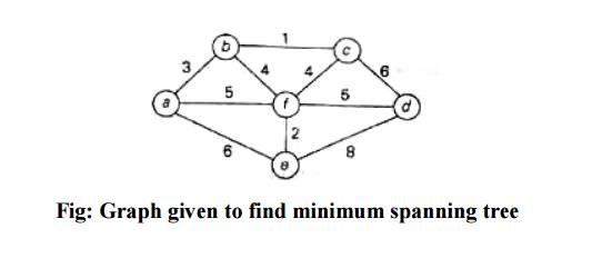
The following figure demonstrates the application of Prim‘s algorithm to a specific graph.

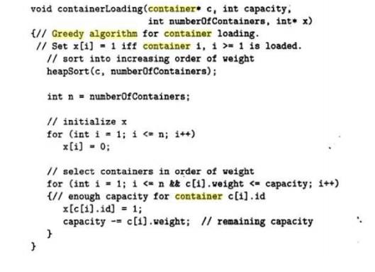
CONTAINER LOADING

The greedy algorithm constructs the loading plan of a single container layer by layer from the bottom up. At the initial stage, the list of available surfaces contains only the initial surface of size L x W with its initial position at height 0. At each step, the algorithm picks the lowest usable surface and then determines the box type to be packed onto the surface, the number of the boxes and the rectangle area the boxes to be packed onto, by the procedure select layer.

The procedure select layer calculates a layer of boxes of the same type with the highest evaluation value. The procedure select layer uses breadth-limited tree search heuristic to determine the most promising layer, where the breadth is different depending on the different depth level in the tree search. The advantage is that the number of nodes expanded is polynomial to the maximal depth of the problem, instead of exponentially growing with regard to the problem size. After packing the specified number of boxes onto the surface according to the layer arrangement, the surface is divided into up to three sub-surfaces by the procedure divide surfaces.

Then, the original surface is deleted from the list of available surfaces and the newly generated sub-surfaces are inserted into the list. Then, the algorithm selects the new lowest usable surface and repeats the above procedures until no surface is available or all the boxes have been packed into the container. The algorithm follows a similar basic framework.

The pseudo-code of the greedy algorithm is given by the greedy heuristic procedure.

procedure greedy heuristic()

list of surface := initial surface of L x W at height 0 list of box type := all box types

while (there exist usable surfaces) and (not all boxes are packed) do

select the lowest usable surface as current surface set depth := 0

set best layer := select layer(list of surface, list of box type, depth)

pack best layer on current surface

reduce the number of the packed box type by the packed amount

set a list of new surfaces := divide surfaces(current surface, best layer, list of box type)

delete current surface from the list of surfaces

insert each surface in list of new surfaces into list of surfaces

end while

Given a layer of boxes of the same type arranged by the G4-heuristic, the layer is always packed in the bottom-left corner of the loading surface.

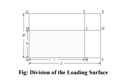
As illustrated in above Figure, up to three sub-surfaces are to be created from the original loading surface by the procedure divide surfaces, including the top surface, which is above the layer just packed, and the possible spaces that might be left at the sides.

If l = L or w = W, the original surface is simply divided into one or two sub-surfaces, the top surface and a possible side surface. Otherwise, two possible division variants exist, i.e., to divide into the top surface, the surface (B,C,E,F) and the surface (F,G,H, I), or to divide into the top surface, the surface (B,C,D, I) and the surface (D,E,G,H).

The divisions are done according to the following criteria, which are similar to those in [2] and [5]. The primary criterion is to minimize the total unusable area of the division variant. If none of the remaining boxes can be packed onto a sub-surface, the area of the sub-surface is unusable. The secondary criterion is to avoid the creation of long narrow strips.

―The underlying rationale is that narrow areas might be difficult to fill subsequently‖. More specifically, if L−l ≥ W −w, the loading surface is divided into the top surface, the surface (B,C,E,F) and the surface (F,G,H, I). Otherwise, it is divided into the top surface, the surface (B,C,D, I) and the surface (D,E,G,H).

Algorithm for Container Loading