Analysis of Algorithm: Fibonacci numbers

Fibonacci numbers

The Fibonacci numbers are defined using the linear recurrence relation

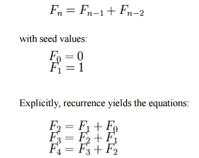
We obtain the sequence of Fibonacci numbers which begins:

0, 1, 1, 2, 3, 5, 8, 13, 21, 34, 55, 89, ...

It can be solved by methods described below yielding the closed form expression which involve powers of the two roots of the characteristic polynomial t² = t + 1; the generating function of the sequence is the rational function t / (1 − t − t²).

Solving Recurrence Equation i. substitution method

The substitution method for solving recurrences entails two steps:

1. Guess the form of the solution.

2.  Use mathematical induction to find the constants and show that the solution works. The name comes from the substitution of the guessed answer for the function when the inductive hypothesis is applied to smaller values. This method is powerful, but it obviously

can be applied only in cases when it is easy to guess the form of the answer. The substitution method can be used to establish either upper or lower bounds on a recurrence. As an example, let us determine an upper bound on the recurrence

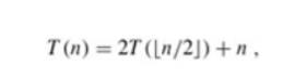
which is similar to recurrences (4.2) and (4.3). We guess that the solution is T (n) = O(n lg n).Our method is to prove that T (n) ≤ cn lg n for an appropriate choice of the constant c > 0. We start by assuming that this bound holds for ⌊n/2⌋, that is, that T (⌊n/2⌋) ≤ c ⌊n/2⌋ lg(⌊n/2⌋).

Substituting into the recurrence yields

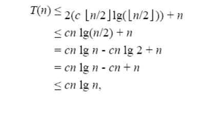
where the last step holds as long as c ≥ 1.

Mathematical induction now requires us to show that our solution holds for the boundary conditions. Typically, we do so by showing that the boundary conditions are suitable as base cases for the inductive proof. For the recurrence (4.4), we must show that we can choose the constant c large enough so that the bound T(n) = cn lg n works for the boundary conditions as well. This requirement can sometimes lead to problems. Let us assume, for the sake of argument, that T (1) = 1 is the sole boundary condition of the recurrence. Then for n = 1, the bound T (n) = cn lg n yields T (1) = c1 lg 1 = 0, which is at odds with T (1) = 1. Consequently, the base case of our inductive proof fails to hold.

This difficulty in proving an inductive hypothesis for a specific boundary condition can be easily overcome. For example, in the recurrence (4.4), we take advantage of asymptotic notation only requiring us to prove T (n) = cn lg n for n ≥ n0, where n0 is a constant of our choosing. The idea is to remove the difficult boundary condition T (1) = 1 from consideration

1. In the inductive proof.

Observe that for n > 3, the recurrence does not depend directly on T

(1). Thus, we can replace T (1) by T (2) and T (3) as the base cases in the inductive proof, letting n0 = 2. Note that we make a distinction between the base case of the recurrence (n = 1) and the base cases of the inductive proof (n = 2 and n = 3). We derive from the recurrence that T (2) = 4 and T (3) = 5. The inductive proof that T (n) ≤ cn lg n for some constant c ≥ 1 can now be completed by choosing c large enough so that T (2) ≤ c2 lg 2 and T (3) ≤ c3 lg 3. As it turns out, any choice of c ≥ 2 suffices for the base cases of n = 2 and n = 3 to hold. For most of the recurrences we shall examine, it is straightforward to extend boundary conditions to make the inductive assumption work for small n.

2. The iteration method

The method of iterating a recurrence doesn't require us to guess the answer, but it may require more algebra than the substitution method. The idea is to expand (iterate) the recurrence and express it as a summation of terms dependent only on n and the initial conditions. Techniques for evaluating summations can then be used to provide bounds on the solution.

As an example, consider the recurrence

T(n) = 3T(n/4) + n.

We iterate it as follows:

T(n) = n + 3T(n/4)

= n + 3 (n/4 + 3T(n/16))

= n + 3(n/4 + 3(n/16 + 3T(n/64)))

= n + 3 n/4 + 9 n/16 + 27T(n/64),

where n/4/4 = n/16 and n/16/4 = n/64 follow from the identity (2.4).

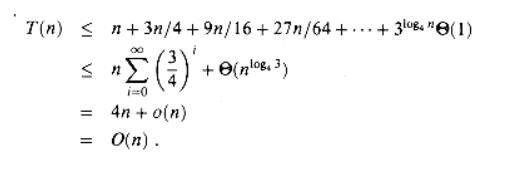
How far must we iterate the recurrence before we reach a boundary condition? The ith term in the series is 3ⁱ n/4ⁱ. The iteration hits n = 1 when n/4ⁱ = 1 or, equivalently, when i exceeds log₄ n. By continuing the iteration until this point and using the bound n/4ⁱn/4ⁱ, we discover that the summation contains a decreasing geometric series:

3. The master method

The master method provides a "cookbook" method for solving recurrences of the form

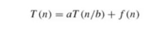
where a ≥  1 and b > 1 are constants and f (n) is an asymptotically positive function.

The master method requires memorization of three cases, but then the solution of many recurrences can be determined quite easily, often without pencil and paper.

The recurrence (4.5) describes the running time of an algorithm that divides a problem of size

n into a subproblems, each of size n/b, where a and b are positive constants. The a subproblems are solved recursively, each in time T (n/b). The cost of dividing the problem and combining the results of the subproblems is described by the function f (n). (That is, using the notation from Section 2.3.2, f(n) = D(n)+C(n).) For example, the recurrence arising from the MERGE-SORT procedure has a = 2, b = 2, and f (n) = Î˜ (n).

As a matter of technical correctness, the recurrence isn't actually well defined because n/b might not be an integer. Replacing each of the a terms T (n/b) with either T (⌊n/b⌋) or T (⌈n/b⌉) doesn't affect the asymptotic behavior of the recurrence, however. We normally find it convenient, therefore, to omit the floor and ceiling functions when writing divide-and- conquer recurrences of this form.