Optimal Binary Search trees

OPTIMAL BINARY SEARCH TREES

A binary search tree's principal application is to implement a dictionary, a set of elements with the operations of searching, insertion, and deletion.

In an optimal binary search tree, the average number of comparisons in a search is the smallest possible.

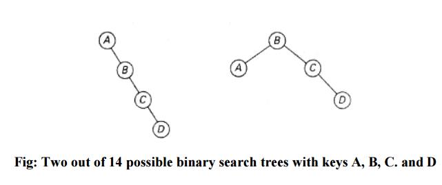
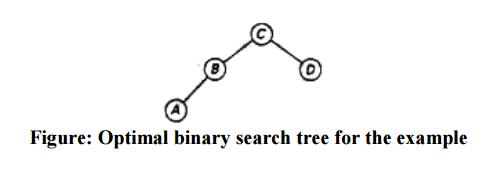
As an example, consider four keys A, B, C, and D to be searched for with probabilities 0.1, 0.2, 0.4, and 0.3, respectively. The above figure depicts two out of 14 possible binary search trees containing these keys. The average number of comparisons in a successful search in the first of this trees is 0.1·1 + 0.2·2 + 0.4·3 + 0.3·4 =2.9 while for the second one it is 0.1·2+0.2·1 +0.4·2+0.3·3 = 2.1. Neither of these two trees is, in fact, optimal.

For this example, we could find the optimal tree by generating all 14 binary search trees with these keys. As a general algorithm, this exhaustive search approach is unrealistic: the total number of binary search trees with n keys is equal to the nth Catalan number which grows to infinity as fast as 4n/n1.5.

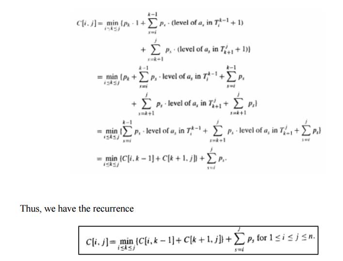
If we count tree levels starting with 1 (to make the comparison numbers equal the keys levels), the following recurrence relation is obtained:

EXAMPLE 1: Let us illustrate the algorithm by applying it to the four-key set.

Key   A       B       C       D

Probability  0.1     0.2     0.4     0.3

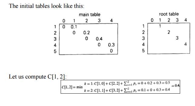
Thus, out of two possible binary trees containing the first two keys, A and B, the root of the optimal tree has index 2 (i.e., it contains B), and the average number of comparisons in a successful search in this tree is 0.4.

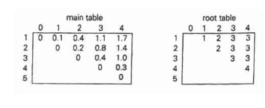
Thus, the average number of key comparisons in the optimal tree is equal to 1.7. Since R[1,

4] = 3, the root of the optimal three contains the third key, i.e., C. Its left subtree is made up of keys A and B, and its right subtree contains just key D.

To find the specific structure of these subtrees, we find first their roots by consulting the root table again as follows. Since R[1, 2] = 2, the root of the optima] tree containing A and B is B, with A being its left child (and the root of the one-node tree: R[1, 1] = 1). Since R[4, 4] = 4, the root of this one-node optimal tree is its only key V. The following figure presents the optimal tree in its entirety.

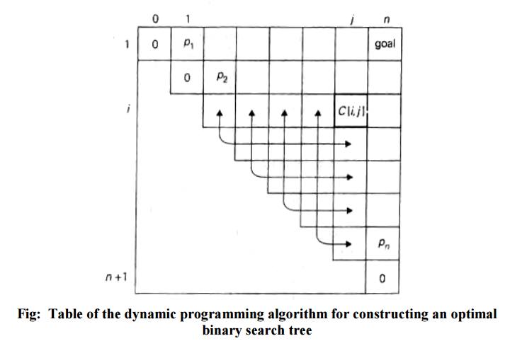
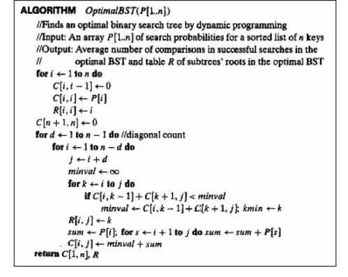
Pseudocode of the dynamic programming algorithm