Dynamic programming

DYNAMIC PROGRAMMING

Dynamic programming is a technique for solving problems with overlapping subproblems. Typically, these subproblems arise from a recurrence relating a solution to a given problem with solutions to its smaller subproblems of the same type. Rather than solving overlapping subproblems again and again, dynamic programming suggests solving each of the smaller subproblems only once and recording the results in a table from which we can then obtain a solution to the original problem.

E.g.  Fibonacci Numbers

0,1,1,2,3,5,8,13,21,34,...,

which can be defined by the simple recurrence

F(0) = 0, F(1)=1. and two initial conditions

F(n) = F(n-1) + F(n-2) for n ≥ 2

GENERAL METHOD -

COMPUTING A BINOMIAL COEFFICIENT

Computing a binomial coefficient is a standard example of applying dynamic programming to a nonoptimization problem.

Of the numerous properties of binomial coefficients, we concentrate on two:

C(n,k) = C(n-1,k-1) + C(n-1,k) for n > k > 0    and

C(n, 0) = C(n, n) = 1.

 Pseudocode for Binomial Coefficient

MULTISTAGE GRAPHS –

ALL PAIR SHORTESET PATH - FLOYD’S ALGORITHM

Given a weighted connected graph (undirected or directed), the all-pair shortest paths problem asks to find the distances (the lengths of the shortest paths) from each vertex to all other vertices. It is convenient to record the lengths of shortest paths in an n-by-n matrix D called the distance matrix: the element d_ij in the ith row and the jth column of this matrix indicates the length of the shortest path from the ith vertex to the jth vertex (1≤ i,j ≤ n). We can generate the distance matrix with an algorithm called Floyd’s algorithm. It is applicable to both undirected and directed weighted graphs provided that they do not contain a cycle of a negative length.

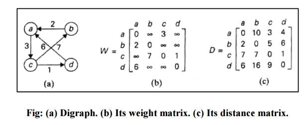
Floyd‘s algorithm computes the distance matrix of a weighted graph with vertices through a series of n-by-n matrices:

Each of these matrices contains the lengths of shortest paths with certain constraints on the paths considered for the matrix. Specifically, the element in the ith row and the jth

column of matrix D (k=0,1,. . . ,n) is equal to the length of the shortest path among all paths from the ith vertex to the jth vertex with each intermediate vertex, if any, numbered not higher than k. In particular, the series starts with D⁽⁰⁾, which does not allow any intermediate vertices in its paths; hence, D⁽⁰⁾ is nothing but the weight matrix of the graph. The last matrix in the series, D⁽ⁿ⁾, contains the lengths of the shortest paths among all paths that can use all n vertices as intermediate and hence is nothing but the distance matrix being sought.

Pseudocode for Floyd’s Algorithms

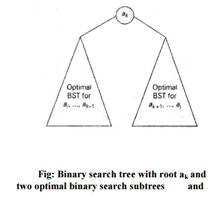
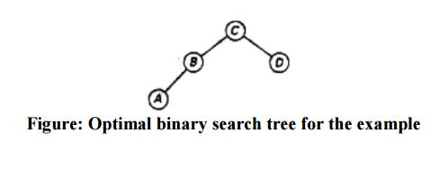
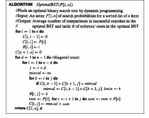
4. OPTIMAL BINARY SEARCH TREES

A binary search tree‗s principal application is to implement a dictionary, a set of elements with the operations of searching, insertion, and deletion.

In an optimal binary search tree, the average number of comparisons in a search is the smallest possible.

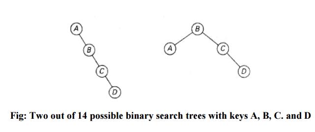
As an example, consider four keys A, B, C, and D to be searched for with probabilities 0.1, 0.2, 0.4, and 0.3, respectively. The above figure depicts two out of 14 possible binary search trees containing these keys. The average number of comparisons in a successful search in the first of this trees is 0.1·1 + 0.2·2 + 0.4·3 + 0.3·4 =2.9 while for the second one it is 0.1·2+0.2·1 +0.4·2+0.3·3 = 2.1. Neither of these two trees is, in fact, optimal.

For this example, we could find the optimal tree by generating all 14 binary search trees with these keys. As a general algorithm, this exhaustive search approach is unrealistic: the total number of binary search trees with n keys is equal to the nth Catalan number which grows to infinity as fast as 4ⁿ/n^1.5.

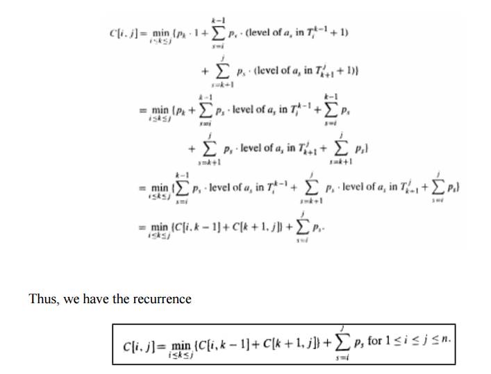
If we count tree levels starting with 1 (to make the comparison numbers equal the keys levels), the following recurrence relation is obtained:

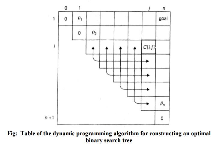
EXAMPLE 1: Let us illustrate the algorithm by applying it to the four-key set.

Key   A       B       C       D

Probability  0.1     0.2     0.4     0.3

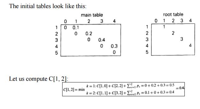
Thus, out of two possible binary trees containing the first two keys, A and B, the root of the optimal tree has index 2 (i.e., it contains B), and the average number of comparisons in a successful search in this tree is 0.4.

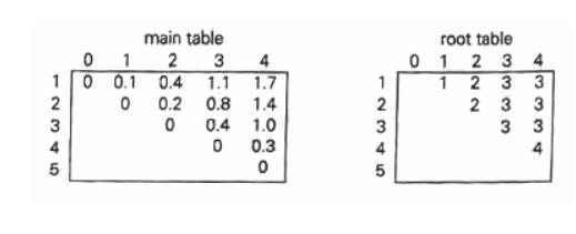
Thus, the average number of key comparisons in the optimal tree is equal to 1.7. Since R[1,

4] = 3, the root of the optimal three contains the third key, i.e., C. Its left subtree is made up of keys A and B, and its right subtree contains just key D.

To find the specific structure of these subtrees, we find first their roots by consulting the root table again as follows. Since R[1, 2] = 2, the root of the optima] tree containing A and B is B, with A being its left child (and the root of the one-node tree: R[1, 1] = 1). Since R[4, 4] = 4, the root of this one-node optimal tree is its only key V. The following figure presents the optimal tree in its entirety.

Pseudocode of the dynamic programming algorithm

5 0/1 KNAPSACK PROBLEM

Let i be the highest-numbered item in an optimal solution S for W pounds. Then S` = S - {i} is an optimal solution for W - w_i pounds and the value to the solution S is V_i plus the value of the subproblem.

We can express this fact in the following formula: define c[i, w] to be the solution for items 1,2, . . . , i and maximum weight w. Then

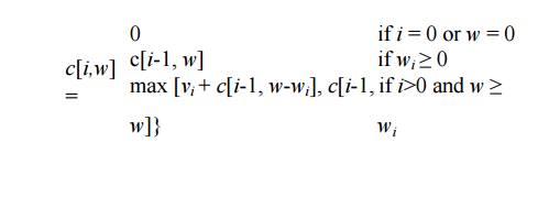
This says that the value of the solution to i items either include i^th item, in which case it is v_i plus a subproblem solution for (i - 1) items and the weight excluding w_i, or does not include i^th item, in which case it is a subproblem's solution for (i - 1) items and the same weight.

That is, if the thief picks item i, thief takes v_i value, and thief can choose from items w - w_i, and get c[i - 1, w - w_i] additional value. On other hand, if thief decides not to take item i, thief can choose from item 1,2, . . . , i- 1 upto the weight limit w, and get c[i - 1, w] value. The better of these two choices should be made.

Although the 0-1 knapsack problem, the above formula for c is similar to LCS formula: boundary values are 0, and other values are computed from the input and "earlier" values of c. So the 0-1 knapsack algorithm is like the LCS-length algorithm given in CLR for finding a longest common subsequence of two sequences.

The algorithm takes as input the maximum weight W, the number of items n, and the two sequences v = <v₁, v₂, . . . , v_n> and w = <w ₁, w_2, . . . , w_n>. It stores the c[i, j] values in the table, that is, a two dimensional array, c[0 . . n, 0 . . w] whose entries are computed in a row-major order. That is, the first row of c is filled in from left to right, then the second row, and so on. At the end of the computation, c[n, w] contains the maximum value that can be picked into the knapsack.

dynamic-0-1-knapsack (v, w, n, w)

for w = 0 to w

do c[0, w] = 0 for i=1 to n

do c[i, 0] = 0 for w=1 to w

do iff w_i ≤ w

then if  v_i + c[i-1, w-w_i]

then c[i, w] = v_i + c[i-1, w-w_i] else c[i, w] = c[i-1, w]

else

c[i, w] = c[i-1, w]

The set of items to take can be deduced from the table, starting at c[n. w] and tracing backwards where the optimal values came from. If c[i, w] = c[i-1, w] item i is not part of the solution, and we are continue tracing with c[i-1, w]. Otherwise item i is part of the solution, and we continue tracing with c[i-1, w-W].

Analysis

This dynamic-0-1-kanpsack algorithm takes θ(nw) times, broken up as follows: θ(nw) times to fill the c-table, which has (n +1).(w +1) entries, each requiring θ(1) time to compute. O(n) time to trace the solution, because the tracing process starts in row n of the table and moves up 1 row at each step.

6. TRAVELING SALESMAN PROBLEM

We will be able to apply the dynamic programming technique to instances of the traveling salesman problem, if we come up with a reasonable lower bound on tour lengths.

One very simple lower bound can be obtained by finding the smallest element in the intercity distance matrix D and multiplying it by the number of cities it. But there is a less obvious and more informative lower bound, which does not require a lot of work to compute.

It is not difficult to show that we can compute a lower bound on the length I of any tour as follows.

For each city i, 1 ≤ i ≤ n, find the sum s_i of the distances from city i to the two nearest cities; compute the sums of these n numbers; divide the result by 2, and, it all the distances are integers, round up the result to the nearest integer:

lb=|S/2|

b) State-space tree of the branch-and- bound algorithm applied to this graph.

(The list of vertices in a node specifies a beginning part of the Hamiltonian circuits represented by the node.)

For example, for the instance of the above figure, formula yields

We now apply the branch and bound algorithm, with the bounding function given by formula, to find the shortest Hamiltonian circuit for the graph of the above figure (a). To reduce the amount of potential work, we take advantage of two observations.

First, without loss of generality, we can consider only tours that start at a.

Second, because our graph is undirected, we can generate only tours in which b is visited before c. In addition, after visiting n-1 = 4 cities, a tour has no choice but to visit the remaining unvisited city and return to the starting one. The state-space tree tracing the algorithm‘s application is given in the above figure (b).

The comments we made at the end of the preceding section about the strengths and weaknesses of backtracking are applicable to branch-and-bound as well. To reiterate the main point: these state-space tree techniques enable us to solve many large instances of difficult combinatorial problems.

As a rule, however, it is virtually impossible to predict which instances will be solvable in a realistic amount of time and which will not.

Incorporation of additional information, such as symmetry of a game‘s board, can widen the range of solvable instances. Along this line, a branch-and- bound algorithm can be sometimes accelerated by knowledge of the objective function‘s value of some nontrivial feasible solution.

The information might be obtainable—say, by exploiting specifics of the data or even, for some problems, generated randomly—before we start developing a state-space tree. Then we can use such a solution immediately as the best one seen so far rather than waiting for the branch-and-bound processing to lead us to the first feasible solution.

In contrast to backtracking, solving a problem by branch-and-bound ha both the challenge and opportunity of choosing an order of node generation and finding a good bounding function.

Though the best-first rule we used above is a sensible approach, it mayor may not lead to a solution faster than other strategies.