Uniformed or Blind search

Uniformed or Blind search

a.     Breadth First Search (BFS)

b.     Depth First Search (DFS)

c.      Depth Limited Search (DLS)

d.     Depth First Iterative Deepening Search (DFIDS)

e.      Bi-Directional Search (BDS)

Breadth First Search (BFS): BFS expands the leaf node with the lowest path cost so far, and keeps going until a goal node is generated. If the path cost simply equals the number of links, we can implement this as a simple queue (“first in, first out”).

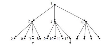
This is guaranteed to find an optimal path to a goal state. It is memory intensive if the state space is large. If the typical branching factor is b, and the depth of the shallowest goal state is d – the space complexity is O(b^d), and the time complexity is O(b^d).

BFS is an easy search technique to understand. The algorithm is presented below. breadth_first_search ()

{

store initial state in queue Q

set state in the front of the Q as current state ;

while (goal state is reached OR Q is empty)

{

apply rule to generate a new state from the current

state ;

if (new state is goal state) quit ;

else if (all states generated from current states are

exhausted)

{

delete the current state from the Q ;

set front element of Q as the current state ;

}

else continue ;

}

}

The algorithm is illustrated using the bridge components configuration problem. The initial state is PDFG, which is not a goal state; and hence set it as the current state. Generate another state DPFG (by swapping 1^st and 2nd position values) and add it to the list. That is not a goal state, hence; generate next successor state, which is FDPG (by swapping 1st and 3rd position values). This is also not a goal state; hence add it to the list and generate the next successor state GDFP.

Only three states can be generated from the initial state. Now the queue Q will have three elements in it, viz., DPFG, FDPG and GDFP. Now take DPFG (first state in the list) as the current state and continue the process, until all the states generated from this are evaluated. Continue this process, until the goal state DGPF is reached.

The 14th evaluation gives the goal state. It may be noted that, all the states at one level in the tree are evaluated before the states in the next level are taken up; i.e., the evaluations are carried out breadth-wise. Hence, the search strategy is called breadth-first search.

Depth First Search (DFS): DFS expands the leaf node with the highest path cost so far, and keeps going until a goal node is generated. If the path cost simply equals the number of links, we can implement this as a simple stack (“last in, first out”).

This is not guaranteed to find any path to a goal state. It is memory efficient even if the state space is large. If the typical branching factor is b, and the maximum depth of the tree is m – the space complexity is O(bm), and the time complexity is O(b^m).

In DFS, instead of generating all the states below the current level, only the first state below the current level is generated and evaluated recursively. The search continues till a further successor cannot be generated.

Then it goes back to the parent and explores the next successor. The algorithm is given below.

depth_first_search ()

{

set initial state to current state ;

if (initial state is current state) quit ;

else

{

if (a successor for current state exists)

{

generate a successor of the current state and

set it as current state ;

}

else return ;

depth_first_search (current_state) ;

if (goal state is achieved) return ;

else continue ;

}

}

Since DFS stores only the states in the current path, it uses much less memory during the search compared to BFS.

The probability of arriving at goal state with a fewer number of evaluations is higher with DFS compared to BFS. This is because, in BFS, all the states in a level have to be evaluated before states in the lower level are considered. DFS is very efficient when more acceptable solutions exist, so that the search can be terminated once the first acceptable solution is obtained.

BFS is advantageous in cases where the tree is very deep.

An ideal search mechanism is to combine the advantages of BFS and DFS.

Depth Limited Search (DLS): DLS is a variation of DFS. If we put a limit l on how deep a depth first search can go, we can guarantee that the search will terminate (either in success or failure).

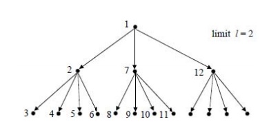
If there is at least one goal state at a depth less than l, this algorithm is guaranteed to find a goal state, but it is not guaranteed to find an optimal path. The space complexity is O(bl), and the time complexity is O(b^l).

Depth First Iterative Deepening Search (DFIDS): DFIDS is a variation of DLS. If the lowest depth of a goal state is not known, we can always find the best limit l for DLS by trying all possible depths l = 0, 1, 2, 3, … in turn, and stopping once we have achieved a goal state.

This appears wasteful because all the DLS for l less than the goal level are useless, and many states are expanded many times. However, in practice, most of the time is spent at the deepest part of the search tree, so the algorithm actually combines the benefits of DFS and BFS.

Because all the nodes are expanded at each level, the algorithm is complete and optimal like BFS, but has the modest memory requirements of DFS. Exercise: if we had plenty of memory, could/should we avoid expanding the top level states many times?

The space complexity is O(bd) as in DLS with l = d, which is better than BFS. The time complexity is O(b^d) as in BFS, which is better than DFS.

Bi-Directional Search (BDS): The idea behind bi-directional search is to search simultaneously both forward from the initial state and backwards from the goal state, and stop when the two BFS searches meet in the middle.

This is not always going to be possible, but is likely to be feasible if the state transitions are reversible. The algorithm is complete and optimal, and since the two search depths are ~d/2, it has space complexity O(b^d/2), and time complexity O(b^d/2). However, if there is more than one possible goal state, this must be factored into the complexity.

Repeated States: In the above discussion we have ignored an important complication that often arises in search processes – the possibility that we will waste time by expanding states that have already been expanded before somewhere else on the search tree.

For some problems this possibility can never arise, because each state can only be reached in one way.

For many problems, however, repeated states are unavoidable. This will include all problems where the transitions are reversible, e.g.

The search trees for these problems are infinite, but if we can prune out the repeated states, we can cut the search tree down to a finite size, We effectively only generate a portion of the search tree that matches the state space graph.

Avoiding Repeated States: There are three principal approaches for dealing with repeated states:

Ø Never return to the state you have just come from

The node expansion function must be prevented from generating any node successor that is the same state as the node’s parent.

Ø Never create search paths with cycles in them

The node expansion function must be prevented from generating

any node successor that is the same state as any of the node’s ancestors.

Ø Never generate states that have already been generated before

This requires that every state ever generated is remembered, potentially resulting in space complexity of O(b^d).

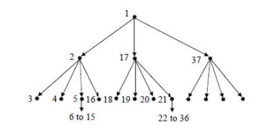
Comparing the Uninformed Search Algorithms: We can now summarize the properties of our five uninformed search strategies:

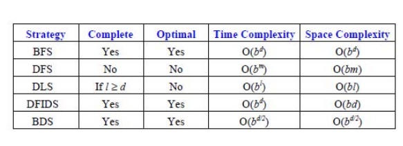
Simple BFS and BDS are complete and optimal but expensive with respect to space and time.

DFS requires much less memory if the maximum tree depth is limited, but has no guarantee of finding any solution, let alone an optimal one. DLS offers an improvement over DFS if we have some idea how deep the goal is.

The best overall is DFID which is complete, optimal and has low memory requirements, but still exponential time.