Mathematics - The concept of derivative | 11th Mathematics : UNIT 10 : Differential Calculus: Differentiability and Methods of Differentiation
Chapter: 11th Mathematics : UNIT 10 : Differential Calculus: Differentiability and Methods of Differentiation
The concept of derivative
The concept of derivative
Calculus grew out of four major problems that mathematicians were working on during the seventeenth century.
1) The tangent line problem
2) The velocity and acceleration problem
3) The minimum and maximum problem
4) The area problem
We take up the above problems 1 and 2 for discussion in this chapter while the last two problems are dealt with in the later chapters.
1) The tangent line problem
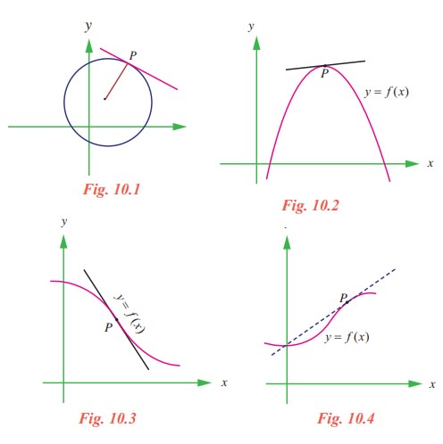
What does it mean to say that a line is tangent to a curve at a point? For a circle, the tangent line at a point P is the line that is perpendicular to the radial line at a point P, as shown in fig. 10.1.
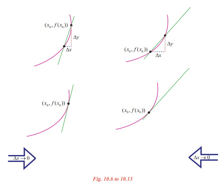
For a general curve, however, the problem is more difficult, for example, how would you define the tangent lines shown in the following figures 10.2 to 10.4.
You might say that a line is tangent to a curve at a point P if it touches, but does not cross, the curve at point P. This definition would work for the first curve (Fig. 10.2), but not for the second (Fig. 10.3). Or you might say that a line is tangent to a curve if the line touches or intersects the curve exactly at one point. This definition would work for a circle but not for more general curves, as the third curve shows (Fig. 10.4).
Essentially, the problem of finding the tangent line at a point P boils down to the problem of finding the slope of the tangent line at point P. You can approximate this slope using a secant line through the point of tangency and a second point on the curve as in the following Fig. 10.5.
Let P(x0, f(x0)) be the point of tangency and Q(x0 + ∆x, f(x0 + ∆x)) be the second point.
The slope of the secant line through the two points is given by substitution into the slope formula
The right hand side of this equation is a difference quotient. The denominator ∆x is the change in x (increment in x), and the numerator ∆y = f(x0 + ∆x) - f(x0) is the change in y.
The beauty of this procedure is that you can obtain more and more accurate approximations of the slope of the tangent line by choosing points closer and closer to the point of tangency.
Tangent line approximation
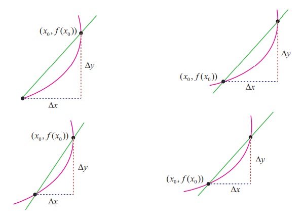
Illustration 10.1
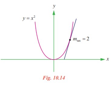
Let us make an attempt to find the slope of the tangent line to the graph of f ( x) = x2at (1, 1). As a start, let us take ∆x = 0.1 and find the slope of the secant line through (1,1) and (1.1, (1.1)2 ).
(i) f(1.1) = (1.1)2 = 1.21
(ii) ∆y = f(1.1) - f(1) = 1.21 - 1 = 0.21
(iii) ∆y/∆x = 0.21 / 0.1 = 2.1
Tabulate the successive values to the right and left of 1 as follows :
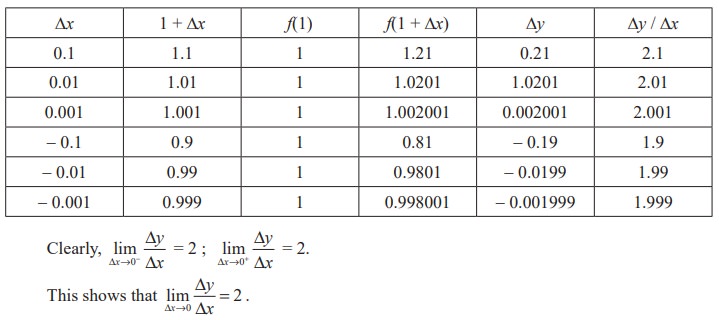
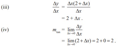
Thus the slope of the tangent line to the graph of y = x2 at (1, 1) is mtan = 2.
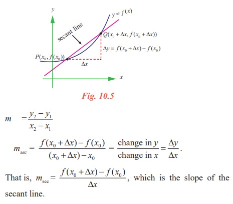
On the basis of the Fig.10.6 to 10.13, Illustration 10.1, and our intuition, we are prompted to say that if a graph of a function y = f(x) has a tangent line L at a point P, then L must be the line that is the limit of the secants PQ through P and Q as Q → P (∆x → 0). Moreover, the slope mtan of L should be the limiting value of the values msec as ∆x → 0. This is summarised as follows:
Definition 10.1 (Tangent line with slope m)
Let f be defined on an open interval containing x0, and if the limit
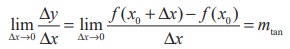
exists, then the line passing through (x0, f(x0)) with slope m is the tangent line to the graph of f at the point (x0, f(x0)).
The slope of the tangent line at (x0, f(x0)) is also called the slope of the curve at that point.
The definition implies that if a graph admits tangent line at a point (x0, f(x0)) then it is unique since a point and a slope determine a single line.
The conditions of the definition can be formulated in 4 steps :
(i) Evaluate f at x0 and x0 + ∆x : f(x0) and f(x0 + ∆x)
(ii) Compute ∆y : ∆y = f(x0 + ∆x) - f(x0)
(iii) Divide ∆y by ∆x (≠ 0) : 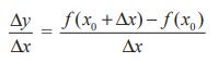
(iv) Compute the limit as ∆x→0 : mtan = 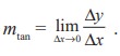
The computation of the slope of the graph in the Illustration 10.1 can be facilitated using the definitions.
(i) f(1) = 12 = 1. For any ∆x ≠ 0
f(1 + ∆x) = (1 + ∆x)2 = 1 + 2∆x + (∆x)2
(ii) ∆y = f(1 + ∆x) - f(1) = 2∆x + (∆x)2 = ∆x (2 + ∆x)
Example 10.1
Find the slope of the tangent line to the graph of f(x) = 7x + 5 at any point (x0, f(x0)).
Solution
Step (i) f(x0) = 7x0 + 5.
For any ∆x≠0 ,
f(x0 + ∆x) = 7(x0 + ∆x) + 5
= 7x0 + 7∆x + 5
Step (ii)
∆y = f(x0 + ∆x) - f(x0)
= (7x0 + 7∆x + 5) − (7x0 + 5)
= 7∆x
Step (iii)
∆y/∆x = 7
Thus, at any point on the graph of f(x) = 7x + 5, we have
Step (iv)
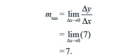
= 7.
Note that for a linear graph, ∆y/∆x is a constant, depends neither on x0 nor on the increment ∆x.
Example 10.2
Find the slope of tangent line to the graph of f(x) = - 5x2 + 7x at (5, f(5)).
Solution
Step (i)
f(5) = - 5(5)2 + 7 × 5 = - 125 + 35 = - 90.
For any ∆x≠ 0 ,
f(5 + ∆x) = - 5(5 + ∆x)2 + 7(5 + ∆x) = - 90 - 43∆x - 5(∆x)2.
Step (ii)
∆y = f(5 + ∆x) - f(5)
= - 90 - 43∆x - 5(∆x)2 + 90 = - 43∆x - 5(∆x)2
= ∆x [- 43 - 5∆x].
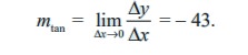
Step (iii)
∆y/∆x = - 43 - 5∆x
Step (iv)
2)Velocity of Rectilinear motion
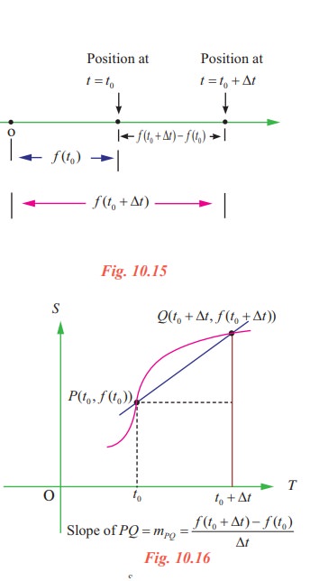
Suppose an object moves along a straight line according to an equation of motion s = f(t), where s is the displacement (directed distance) of the object from the origin at time t. The function f that describes the motion is called the position function of the object. In the time interval from t = t0 to t = t0 + ∆t, the change in position is f(t0 + ∆t) - f(t0). The average velocity over this time interval is
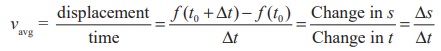
which is same as the slope of the secant line PQ in fig. 10.16.
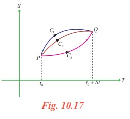
In this time interval ∆t (from t0 to t0 + ∆t) the motion may be of entirely different types for the same distance covered (traversed). This is illustrated graphically by the fact that we can draw entirely different curves C1, C2, C3 ... between the points P and Q in the plane. These curves are the graphs of quite different motions in the given time intervals, all the motions having the same average velocity ∆s/∆t.
Now suppose we compute the average velocities over shorter and shorter time intervals [t0, t0 + ∆t]. In other words, we let ∆t approach 0. Then we define the velocity (or instantaneous velocity) v(t0) at time t = t0 as the limit of these average velocities.
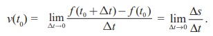
This means that the velocity at time t = t0 is equal to the slope of the tangent line at P.
Illustration 10.2
The distance s travelled by a body falling freely in a vacuum and the time t of descent are variables. They depend on each other. This dependence is expressed by the law of the free fall:
s= 1/2 gt2 (absence of initial velocity), g is the gravitational constant.
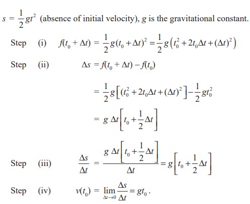
It is clear from this that the velocity is completely defined by the instant t0. It is proportional to the time of motion (of the fall).
3) The derivative of a Function
We have now arrived at a crucial point in the study of calculus. The limit used to define the slope of a tangent line or the instantaneous velocity of a freely falling body is also used to define one of the two fundamental operations of calculus – differentiation.
Definition 10.2
Let f be defined on an open interval I ⊆ R containing the point x0, and suppose that 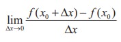 exists. Then f is said to be differentiable at x0 and the derivative of f at x0, denoted by f ′(x0 ) , is given by
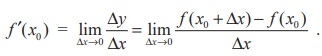
For all x for which this limit exists,
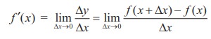
is a function of x.
Be sure you see that the derivative of a function of x is also a function of x. This “new” function gives the slope of the tangent line to the graph of f at the point (x, f(x)), provided the graph has a tangent line at this point.
The process of finding the derivative of a function is called differentiation. A function is differentiable at x if its derivative exists at x and is differentiable on an open interval (a, b) if it is differentiable at every point in (a, b).
In addition to f ′(x) , which is read as ‘f prime of x’ or ‘f dash of x’, other notations are used to denote the derivative of y = f(x). The most common notations are
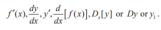
Herer d/dx or D is the differential operator.
The notation dy/dx is read as “derivative of y with respect to x” or simply “dy - dx”, or we should rather read it as “Dee y Dee x” or “Dee Dee x of y”. But it is cautioned that we should not regard dy/dx as the quotient dy ÷ dx and should not refer it as “dy by dx”. The symbol dy/dx is known as Leibnitz symbol.
4) One sided derivatives (left hand and right hand derivatives)
For a function y = f(x) defined in an open interval (a, b) containing the point x0, the left hand and right hand derivatives of f at x = x0 are respectively denoted by f ′(x0− ) and f ′(x0+ ), are defined as
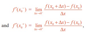 , provided the limits exist.
That is, the function is differentiable from the left and right. As in the case of the existence of limits of a function at x0 , it follows that
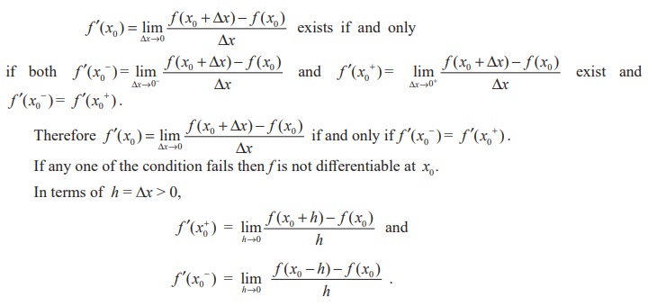
Definition 10.3
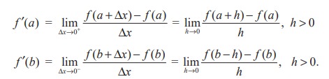
A function f is said to be differentiable in the closed interval [ a , b] if it is differentiable on the open interval ( a , b) and at the end points a and b,
If f is differentiable at x = x0 , then 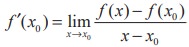 , where x = x0 + ∆x and ∆x → 0 is equivalent to x → x0 . This alternative form is some times more convenient to be used in computations.
As a matter of convenience, if we let h = ∆x, then 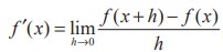 , provided the limit exists.
Related Topics