Numerical solution methods for natural frequencies and mode shapes

Numerical solution methods for natural frequencies and mode shapes in relation to structural dynamics during earthquakes

Abstract: This chapter discusses basic solution schemes as well as approximate methods for finding natural frequencies and mode shapes. The methods include Vianelloâ€'Stoodala power method, transfer matrix method, Jacobi method, Holzer method, Rayleigh’s approximation and Dunkerley’s approximation. Some of the approximate methods will lead to upper bound solutions and some lower bound solutions. A relevant program in MATHEMATICA is also given.

Key words: banded matrix, sweeping technique, deflation, transfer matrix, Holzer method.

Introduction

The important step in the dynamic analysis of a multiple-degrees-of-freedom (MDOF) system is quite often the solution of the eigenvalue problem, or the determination of the system natural frequencies and the corresponding normal vibration modes. This is particularly true if a mode superposition analysis is to be conducted. Several procedures for solving the eigenvalue problem have been discussed in many books. Predicting or finding the roots of the characteristic polynomial as discussed in Chapter 10 is satisfactory only for systems having few degrees of freedom. For large MDOF systems, extracting the roots of the characteristic polynomial requires computational effort and is quite often an indeterminable task. This chapter discusses the basic solution schemes as well as approximate methods for finding frequencies.

General solution methods for eigen problems

In structural dynamics, the basic eigen problem for an MDOF system having ‘n’ degrees of freedom is represented as

[k]{φ} = λ[m]{φ}                        …  . . . . 11.1

Let [k] be the stiffness matrix of order ‘n’ and [m], the mass matrix, also of order ‘n’. For most structural systems, [k] is normally banded matrix and [m] is a diagonal matrix for a lumped mass formulation (without rotary inertia) coupling or a narrowly banded matrix for a consistent mass formulation.

There are ‘n’ eigenvalues and ‘n’ eigenvectors satisfying the above equation. The rth eigen pair is determined by (λ_r,{φ}_r). In dynamic problems, the eigenvalues are the square of the natural frequencies ω _n² such that

0 < λ₁ < λ₂ <…< λ_{n           ……….  .. .} 11.2

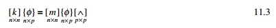
The dynamic response of MDOF systems having a large number of degrees of freedom is generally confined to a relatively small subset of the lowest vibration modes of the system. Therefore for such systems, only ‘p’ eigen pairs need to be solved for where p << n. The solution of p eigen values and the corresponding eigenvectors can be written as

The majority of the eigen problem solution techniques can be classified as

•       vector iteration methods;

•       transformation methods;

•       polynomial iteration methods.

Clearly all the methods are iterative in nature because the solution of the eigen problem as defined in Eq. 11.1 is tantamount to solving the characteristic polynomial of order ‘n’. Since explicit formulas for the determination of roots to the characteristic polynomial having an order higher than 4 do not exist, an iterative solution is mandatory.

The main essence of each method is very distinctive. The vector iteration methods are based on the property

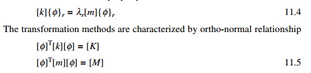
Let [K] and [M] be modal stiffness and modal mass respectively. The polynomial iteration is based on the property that the characteristic polynomial is a function of λ_r, and

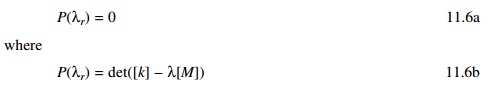
The characteristic polynomial is of order ‘n’. Solution of characteristic polynomial has been discussed in Previous Pages.

Vector iteration technique

1  Vianello and Stoodala method (power method)

This iterative method can be applied to extract the highest eigenvalue of either symmetric or unsymmetric matrix of any order. Consider the homogeneous equation written in the form of

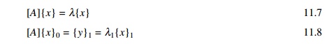
Assume any vector {x}₀ and multiplying with [A] matrix gives {y}₁ can be written in terms of λ₁{x}₁ by taking highest element (associated vector) outside and this can be used in the next iteration as

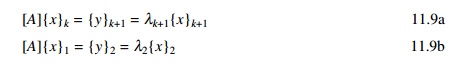
It can be seen that the eigenvalue λ as well as eigenvector will converge. The iteration can be stopped when |λ_n+1 â€' λ_n| < ε (tolerance) and λ is the highest eigenvalue in the absolute sense.

Consider the problem in dynamics

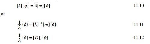
[D]₁ is called the dynamic matrix. Application of the power method will converge to (1/λ)_max or λ_min = λ₁ · λ₁ is called the least dominant eigenvalue and {Ï•}₁ is called least dominant eigenvector. However the method may be modified to calculate eigenvalues and the corresponding eigenvectors for higher modes by matrix deflation or deflation of the iteration vectors.

Assume using the power method we get the (1/λ)_max or λ_min = λ₁ and {φ}₁ pair. The basic premise for vector deflation is that, for an iteration vector to converge to a required eigenvector, the iteration vector must be orthogonal to the eigenvector. Therefore, for this case at hand, this can be interpreted as meaning that if the iterative vector is orthogonalized to the eigenvectors already calculated (for example {φ}₁) the vector is precluded and occurs instead to another (higher) eigenvector. More succinctly, an eigen pair other than (λ₁, {φ}₁) becomes the least dominant eigen pair.

2  Method 1 sweeping technique

To find the second eigenvalue assume a trial vector that is a linear combination of all eigenvectors.

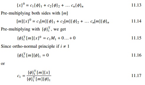
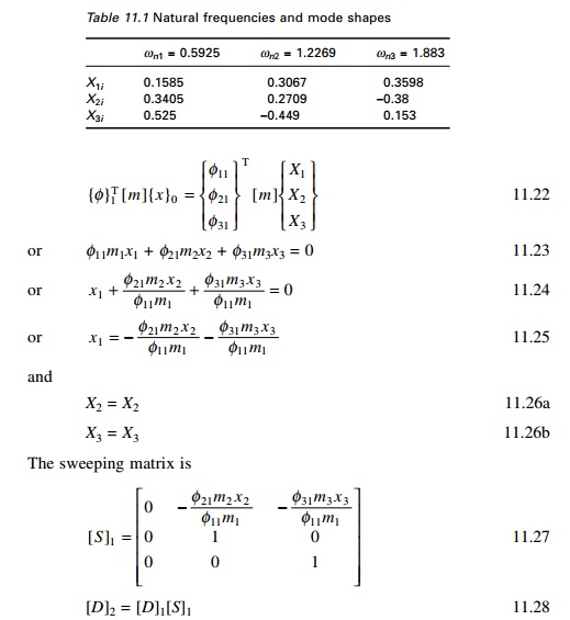
In the trial vector assumed in Eq. 11.13, let us sweep out the effect of mode 1 as

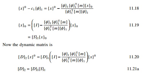
If {φ}₁ is the normalized eigenvector, as proved in Chapter 10, {φ }₁^T [ m]{φ}₁ = 1 because of the normalization principle. In that case dynamic matrix is written as [D]₂ = [D]₁[S]₁ where [S]₁ is given as in Eq. 11.18 as

In Eq. 11.19, [S]₁ is called sweeping matrix for the first mode. The purpose of [S]₁ is to eliminate or sweep out the effect of mode 1. Similarly [S]_n is to sweep out the effect of modes for 1 to n and allow the mode (n + 1) to become least dominant.

3  Method 2 â€' deflation method

Assume we find (λ₁, {φ}₁) pair to obtain some eigenvalue using the ortho-normal principle.

The power method will converge to the second eigenvalue and the corresponding normalized eigenvector {Ï•}₂ can be obtained.

To extract the third eigenvalue,

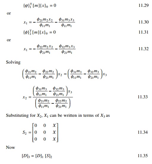
Using the power method, the iteration will converge to third eigenvalue and the corresponding normalized eigenvector can be obtained.

Let us use the same example and assume we obtain the highest eigenvalue as 2.8453 and the corresponding normalized eigenvector as given in method 1. Substituting the corresponding values in Eq. 11.25, we get

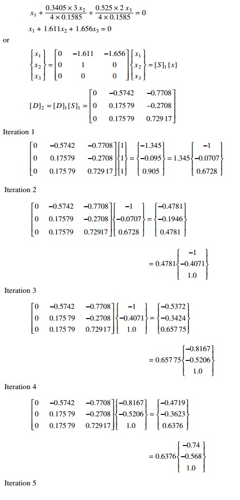
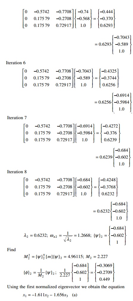
Using the first normalized eigenvector we obtain the equation

x₁ = â€'1.611x₂ â€' 1.656x₃  (a)

Using the second normalized eigenvector we obtain the equation

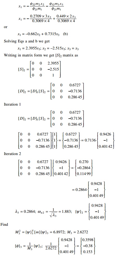
The procedure can be programmed very easily in the EXCEL package.

Jacobi’s method

The matrix iteration method discussed in Section 11.3 produces the eigenvalues and eigenvectors of matrix [D]₁ one at a time. Jacobi’s method is also an iterative method but produces all the eigenvalues and eigenvectors of the matrix [D]₁ simultaneously. [D]₁ is a real symmetrix matrix and has only real eigenvalues. There is an orthogonal matrix [R] such that [R]^T[D]₁[R] is a diagonal matrix. The diagonal elements are the eigenvalues and the columns of [R] is generated as a product of several rotation matrices as

[R] = [R₁][R₂][R₃]…  ---- 11.36

Consider the highest off-diagonal term of matrix [D]₁. Let it be d_ij. Find

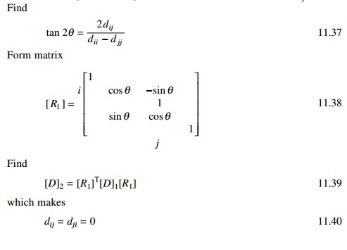
Again find the highest off-diagonal term and form [R₂] matrix. While making this off-diagonal term as zero, it introduces non-zero contributions to formerly zero positive. However, successive matrices of the form

[R₂]^T[R₁]^T[D]₁[R₁][R₂]                    - - - - - - 11.41

[R₃]^T[R₂]^T[R₁]^T[D]₁[R₁][R₂][R₃]                 - - - - - - 11.42

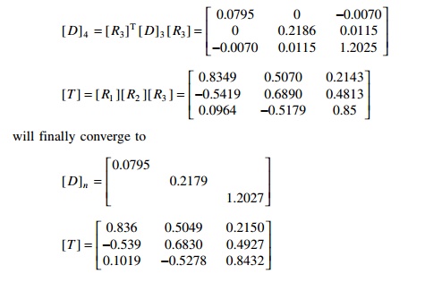
converges to the required diagonal form. Find matrix [R] such that

[R] = [R₁][R₂][R₃]…[R_n]               - - - - - - 11.43

is the required eigenvector.

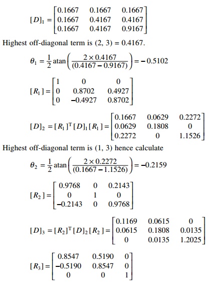
Consider Example 11.1 with mass matrix as [I]. The dynamic matrix is written as

Transfer matrix method to find the fundamental frequency of a multi-storeyed building (shear frame)

Consider a shear frame shown in Fig. 11.1 consisting of ‘n’ storeys. Consider the free body diagram of the ith storey as shown in Fig. 11.2. Here ‘m’ is the mass, ‘k’ is the stiffness, ‘V’ is the shear, ‘ω’ is the natural frequency and ‘v’ is the displacement.

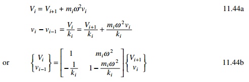
Considering inertia force, the shear in the ith storey can be written in terms of shear of (i+1)th storey.

Initially the displacement at the top storey level and the natural frequency are both assumed. By using the transfer matrix method, it is possible to find the displacement at the base as well as shear in the base storey. If the support displacement is not zero, a new value for the natural frequency is assumed and the procedure is repeated till we get the value of the base displacement as zero.

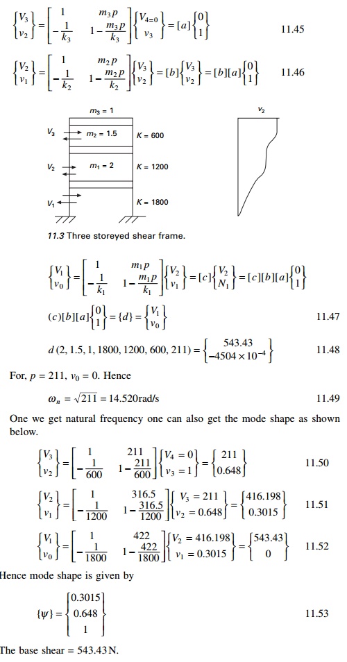
Example 11.2

Find the natural frequency of the three storeyed shear building as shown in Fig. 11.3, given the mass and the stiffness.

Solution

Since ‘MATHEMATICA’ can solve the problem using symbolic processing, we will write in symbolic form. Transfer matrix at top frame ( assume p = ω _n² )

One we get natural frequency one can also get the mode shape as shown below.

Holzer method for torsional vibrations

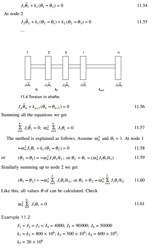
The Holzer method falls under the determinant search technique. The method can be applied to rectilinear or angular motions for damped as well as undamped systems. The method is best suited for systems where the components are arranged along the basic axis. Let us consider the torsional vibration for shafts as shown in Fig. 11.4.

The torsional moment equilibrium at node 1 can be written as

Approximate methods for finding the natural frequencies

1  Rayleigh’s quotient

In many practical situations involving MDOF systems, only the accurate estimation of the fundamental frequency is required. In such cases, laborious calculations to extract all the normal vibration modes of the system are not warranted and the approximate methods are desirable. This section discusses two approximate methods for estimating the fundamental frequency of MDOF systems.

The first method, Rayleigh’s method, is an upper bound method based on energy principles and stiffness approach. The second method, Dunkerley’s approximation, is based on the flexibility of the system eigenvalue problem and therefore provides lower bound estimation of the fundamental frequency. Thus the upper bound estimation of the fundamental frequency provided by Rayleigh’s method can be complemented by the lower bound estimation afforded by Dunkerley’s approximations to envelope true fundamental frequency.

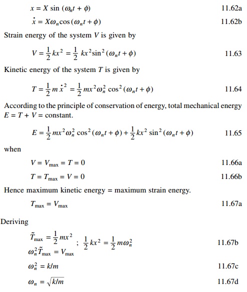
Consider that an undamped single-degree-of-freedom (SDOF) mass spring system is in free harmonic motion given by

2  Rayleigh’s quotient method to MDOF

In the above we have discussed Rayleigh’s method to determine the fundamental frequency of an SDOF system. Application of the Rayleigh’s method to determine the fundamental frequency of an MDOF system is presented in this section.

Consider the eigenvalue problem of the MDOF system represented by equation

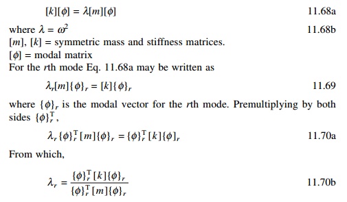
In Eq. 11.70b, the denominator is related to the kinetic energy for the rth mode and the numerator is related to the potential energy, or the strain energy of the rth mode. If the modal vector {φ}_r is replaced with any arbitrary vector {A}, Eq. 11.70b is written as

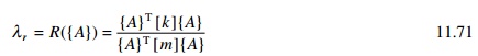
where R({A}) is a scalar quantity referred to as Rayleigh’s quotient. It is evolved from Eq. 7.51 that Rayleigh’s quotient is dependent upon the known matrix [m] and [k] and the unknown arbitrary vector {A}. Obviously if {A}

coincides with one of the systems normal modes then λ_R is the corresponding eigenvalue or normal frequency of the system. A very important property of Rayleigh’s quotient is

and it also follows that for any vector {A}, if [K] is positive definite, R({A}) > 0. If [K] is positive semi-definite,

Equation 11.65 thus indicates that the Rayleigh’s quotient is never lower than the fundamental eigenvalue, and furthermore the minimum value the Rayleigh’s quotient can assume is that of the fundamental eigenvalue itself. Therefore, Rayleigh’s quotient is very good technique to estimate the fundamental frequency of MDOF systems. A reasonable estimate for the vector {A} corresponding to the fundamental mode is the vector of static displacement resulting from subjecting the masses in the system to forces proportional to their weights. Many seismic design code present expressions to estimate the fundamental frequency of high-rise building based on this concept. The natural frequency thus obtained is called the Rayleigh frequency ω_R expressed as

The accuracy of the Rayleigh frequency ω_R depends entirely on the displacement vector {A} used to represent the vibration mode shape. In principle, any vector {A} may be selected which satisfies the geometric boundary conditions. However, any vector other than the true modal vector requires the action of additional external constraints to maintain equilibrium, which would in turn stiffen the structure, resulting in increased computed frequency. Therefore the true vibration mode will yield the lowest frequency

obtained by Rayleigh’s method. Hence the approximation yielding the lowest frequency for a particular case is the best result.

Steps

1.     Estimate the fundamental mode of vibration. This may be done either by assuming the displacement of the modes directly or computing the displacement from the associated forces.

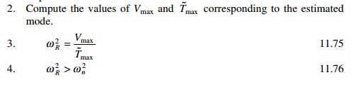
If the frequency is computed for several displacement-assumed configurations, the smallest of the computed values will be close to the exact value of ω_n and the associated configuration is closest to the actual configuration.

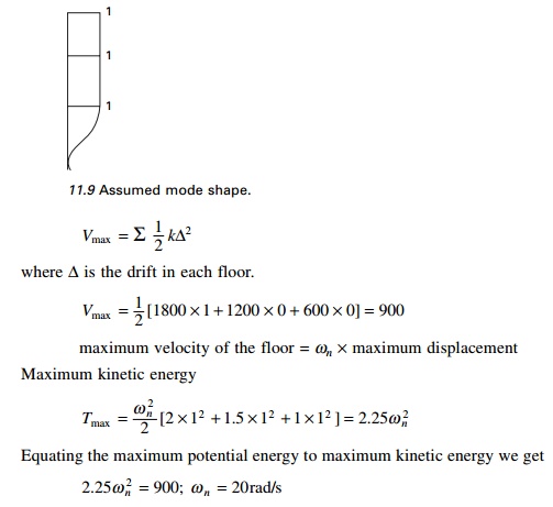
Example 11.6

Determine the fundamental frequency of the shear frame shown in Fig. 11.3 by the improved Rayleigh method.

Solution

R00 method

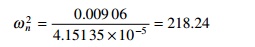
Assume the mode shape as shown in Fig. 11.9. Maximum potential energy:

R₀₁ method

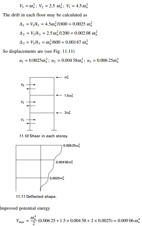
By calculating the shear in each floor let us improve the mode shape. The shear in each floor can be calculated as (see Fig. 11.10)

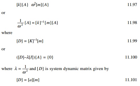
Equating this improved potential energy to previously calculated kinetic energy

0.009 06 ω _n⁴  = 2.25ω _n²

Or

ω _n²  = 234.375; ω _n  = 15.309

R₁₁ method

Improve the kinetic energy. Velocity at each storey level:

v₁  = 0.0025 ω _n³ ; v ₂  = 0.004 58 ω _n³ ; v₃  = 0.006 25 ω _n³

T_{max(improved)}  = ω _n⁶ /2[2 Ã- 0.0025²  + 1.5 Ã- 0.004 58²  + 1 Ã- 0.006 25² ]

= 4.15135 Ã- 10 ^âˆ'5 ω _n⁶

Equating maximum kinetic energy to maximum potential energy, we get

0.009 06 ω _n⁴  = 4.15135 Ã- 10 ^âˆ'5 ω _n⁶

ω_n = 14.77rad/s

Dunkerley’s approximation

It is another approximate method for estimating the fundamental frequency for MDOF systems. The method yields accurate results for systems for which

damping is negligible and the natural frequencies are well separated. Dunkerley’s equation provides a ‘lower bound’ estimate with fundamental frequency and is therefore complementary with the Rayleigh method that provides an ‘upper bound’ estimate with fundamental frequency.

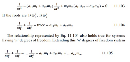
To derive Dunkerley’s equation consider the equation

where [a] is the flexibility matrix.

The frequency equation is obtained by expanding the determinant of the characteristic matrix in Eq. 11.101.

Let us consider a two-degrees-of-freedom system with lumped mass diagonal matrix. Thus the resulting characteristic determinant becomes

Expanding Eq. 11.102 results in the system frequency equation, i.e. second order equation in λ = 1/ω² given by,

If the roots are 1/ ω₁² , 1/ ω ₂²

The relationship represented by Eq. 11.104 also holds true for systems having ‘n’ degrees of freedom. Extending this ‘n’ degrees of freedom system

Dunkerley’s approximation to the fundamental frequency is made on the assumption that if the fundamental frequency ‘ω’ is much lower than the higher harmonics (ω₂,… ω_n) then the terms on the left hand side 1/ ω ₂² … 1/ ω _n² can be calculated. The elimination of these terms yields an estimate of 1/ ω₁² which is higher than the true value thereby making the estimate of ‘ω₁’ lower than the exact value of fundamental frequency. The Dunkerley’s lower bound estimate of ‘ω₁’ is approximated to

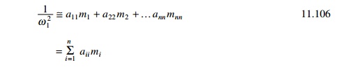
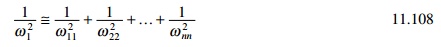
In Eq. 11.106 the term ‘a_iim_i’ represents the contribution of each mass to 1/ω₁² in the absence of all other masses. Thus

where ω _ii² is the natural frequency of an SDOF system with mass ‘m_i’ acting alone at state i. Hence Dunkerley’s equation is given by

Summary

In this chapter the sweeping technique combined with power method and transfer matrix methods have been discussed to find the natural frequencies of n-degrees-of-freedom system. In addition, Rayleigh’s coefficient method and Dunkerley’s approximate methods are also discussed to find the approximate fundamental frequency of an n-degrees-of-freedom system.