Free and forced vibration of a continuous system

Free and forced vibration of a continuous system in relation to structural dynamics during earthquakes

Abstract: A physical system can also be modelled as a continuous system with distributed mass and stiffness. The governing differential equations of distributed systems are partial differential equations. In this page, strings, bars, shafts and beams are modelled as distributed systems and the dynamic response is studied by solving partial differential equations. Relevant programs in MATHEMATICA and MATLAB are also given.

Key words: distributed systems, normal modes, orthogonality, rotary inertia, shear deformation, moving loads.

Introduction

Structures analysed so far have been treated as discrete systems. In discrete systems stiffness and mass as well as damping are modelled as discrete properties. Dynamic analysis of discrete structures will lead to ordinary differential equations which are amenable to numerical solutions. Another method of modelling physical systems is based on the distributed mass and stiffness characteristics. Systems for which stiffness and mass have distributed rather than discrete properties are referred to as distributed systems or continuous systems.

If the system is modelled as a distributed system, the governing differential equations are partial differential equations which are more difficult to solve. The result obtained from a continuous model is more accurate than discrete systems. In this chapter, we shall consider the vibration of simple continuous systems, strings, bars, shafts and beams. It will readily become apparent, however, that analytical or closed form solutions can be obtained only for relatively simple continuous systems with well-defined boundary conditions. In general, the frequency equation of a continuous system is a transcendental equation that yields an infinite number of natural frequencies and normal modes. This is in contrast to the behaviour of discrete systems which yield a finite number of frequencies and mode shapes.

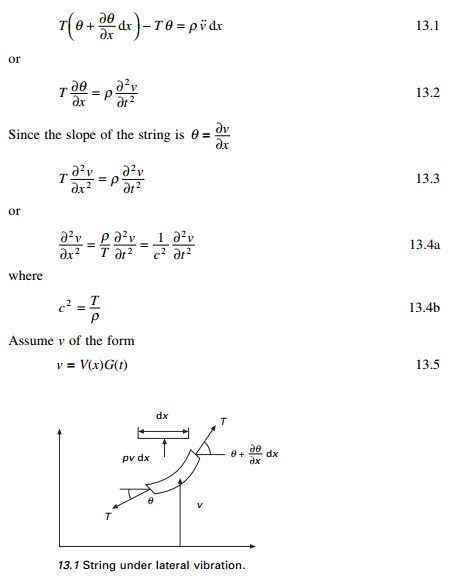
Vibration of a string

Consider a flexible string of mass ρ/unit length is stretched under tension T as shown in Fig. 13.1. The dynamic analysis is carried out based on the following assumptions:

•       lateral deflection v is very small;

•       the change in tension ∆T with deflection is negligible.

Considering vertical equilibrium of forces we get

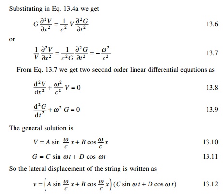
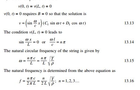
A, B, C and D can be solved depending on initial and boundary conditions. For example if the string is stretched between two fixed points with distance L, the boundary conditions are

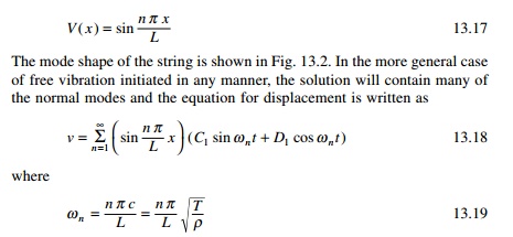
The mode shape of the string is shown in Fig. 13.2. In the more general case of free vibration initiated in any manner, the solution will contain many of the normal modes and the equation for displacement is written as

Fitting the equation to the initial conditions v(x, 0), and v˙ ( x, 0) the values of C_n1, D_n1 can be evaluated.

Longitudinal vibration of a uniform rod

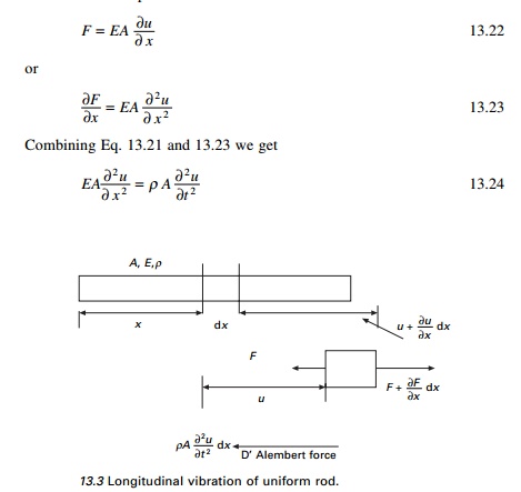
The rod considered in the section is thin and uniform along its length. The rod has cross-sectional area A, modulus of elasticity E and material mass density ρ/unit volume as shown in Fig. 13.3.

The free body diagram of a differential element is shown in Fig. 13.3. In the deformed position the deformed length of dx is dx [1 + (∂u/∂x) dx]. Summing the horizontal forces the equilibrium equation is written as

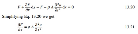
where ∂²u/∂t² is the acceleration of the differential element. Noting that axial force F can be expressed as

Following the initial conditions and the boundary conditions the displacement can be obtained at any time t at any position x.

Example 13.2

Determine expressions for the natural frequencies and displacement response for longitudinal vibration of a uniform rod with one end fixed and the other end free as shown in Fig. 13.4.

Example 13.3

Determine the natural frequencies and mode shapes of a free�'free rod (a rod with both ends free).

Example 13.4

Determine the expression for the natural frequencies and displacement response for longitudinal vibration of a uniform rod with one end fixed and the other end having a concentrated mass M as shown in Fig. 13.7. Determine the expression for the frequency equation of longitudinal vibrations. Length of the rod = L, mass density = ρ, and cross-sectional area = A.

Torsional vibration of shaft or rod

Figure 13.8 represents a non-uniform shaft subjected to an external torque m(x, t)/unit length. If θ (x, t) denotes the angle of twist of the cross-section, the relation between twist and twisting moment M_t (x, t) is given by

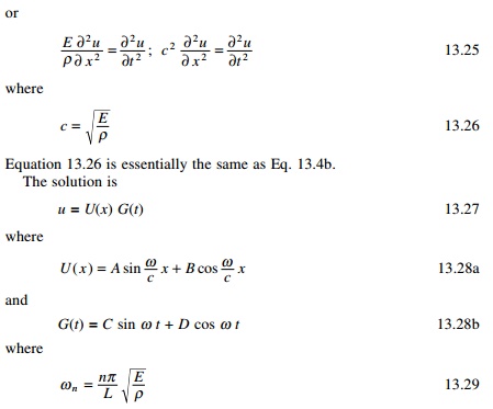
Table 13.1 Values of frequencies ω = λL/c for various ratios of m/M

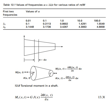
where G is the shear modulus and GJ(x) is the torsional stiffness, with J(x) denoting polar moment of inertia of the cross-section.

If the mass polar moment of inertia of the shaft/unit length is I₀, the inertia torque acting on an element of length dx becomes

If an external torque m_T (x, t) acts on the shaft/unit length, the application of Newton’s second law yields

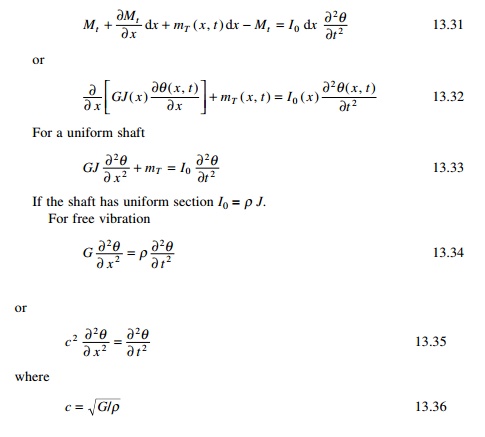
The equation is analogous to the longitudinal vibration of a rod.

If the shaft is given an initial angular displacement θ₀(x) at t = 0, the initial conditions can be stated as

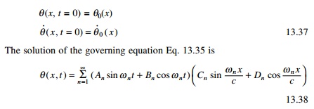
The common boundary conditions for torsional vibration of uniform shaft are indicated in Table 13.2 along with corresponding frequency conditions.

Free flexural vibration of beams

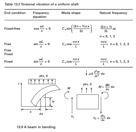
Consider a beam sufficiently long compared with its cross-section so that shear deformations can be ignored. The effect of axial load, shear deformation and rotary inertia will be discussed in the following sections. The free body diagram of a beam segment of element length dx is shown in Fig. 13.9.

Table 13.2 Torsional vibration of a uniform shaft

From the elementary theory of bending of beam (Euler�'Bernoulli theory)

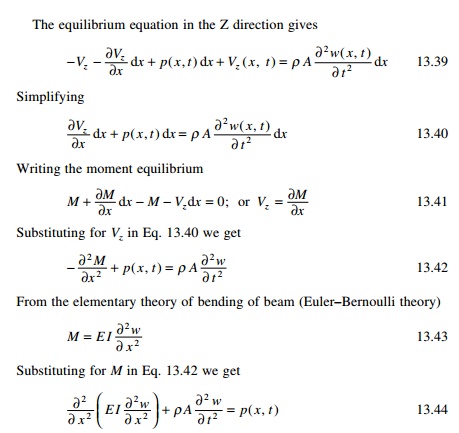
where E is the Young’s modulus and I is the moment of inertia of beam cross-section about y-axis. For free vibration of beams p(x, t) = 0 and hence the equation for free vibration of non uniform beam is written as

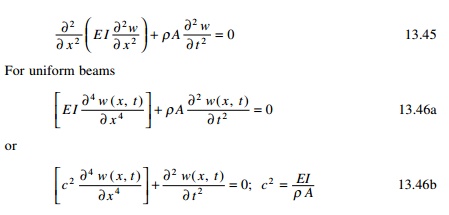
The equation of motion involves a second order derivative with respect to time and a fourth derivative with respect to x and hence two initial conditions and four boundary conditions are necessary to solve the problem. Usually, the values of lateral displacement w₀(x) and w˙ ₀ ( x ) at t = 0 so that initial conditions become

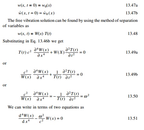
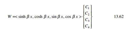
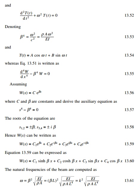
The function W(x) is known as normal mode or characteristic function of the beam and ω is the natural frequency of vibration. For any beam there will be an infinite number of modes with one natural frequency associated with each normal mode. The unknown values C₁, C₂, … C₄ and the value of β can be determined from the boundary conditions of the beam as indicated below.

For a beam of length L the deflection, slope, curvature and d³W/dx³ may be written at the two ends of the beam (x = 0, x = L) as

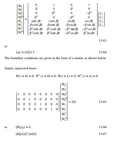
The boundary conditions are given in the form of a matrix as shown below.

Simply supported beam

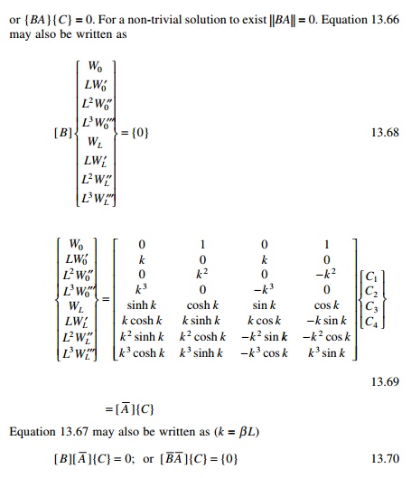
For a non-trivial solution to exist || BA || = 0 and the determinant is a function of k and the root of the equation can be found out. This can very easily be done using the MATHEMATICA package.

Orthogonality of normal modes

The normal function W(x) satisfies Eq. 13.51 as

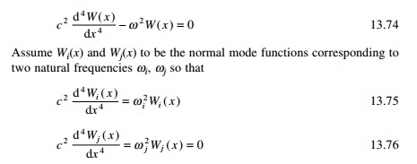
Multiplying Eq. 13.75 by W_j and Eq. 13.76 by W_i we get

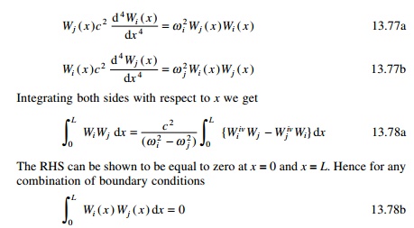
The RHS can be shown to be equal to zero at x = 0 and x = L. Hence for any combination of boundary conditions

orthogonality of normal functions for the transverse vibration of beams.

Effect of axial force (tension or compression)

The study of vibration of beams under the action of axial force finds application in the study of vibration of cables and guy wires. Even though we have treated the cable by an equivalent string, many cables have failed owing to fatigue caused by alternating flexure, which is the result of regular shedding of vortices from the cables due to high wind. Hence it is important to study the vibration of beams due to axial forces.

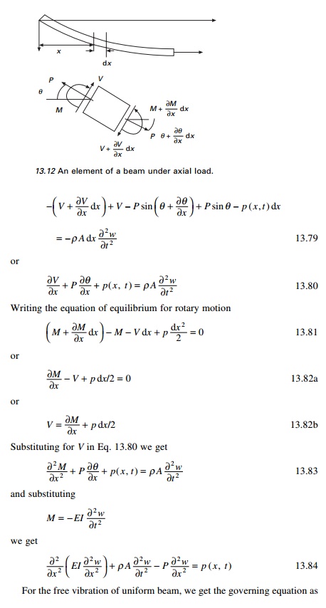
Consider the equation of motion of an element of the beam shown in Fig. 13.12. Writing the equation of equilibrium for vertical motion we get

For a simply supported beam of length L the boundary conditions are

W(0) = W(L) = W″(0) = W″(L) = 0  …………  13.96

Applying the boundary conditions

C₁ = C₂ = C₄ = 0;                and C₃ sin β L = 0     --- 13.97

β L = nπ; n = 1, 2, 3…          --- 13.97

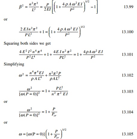
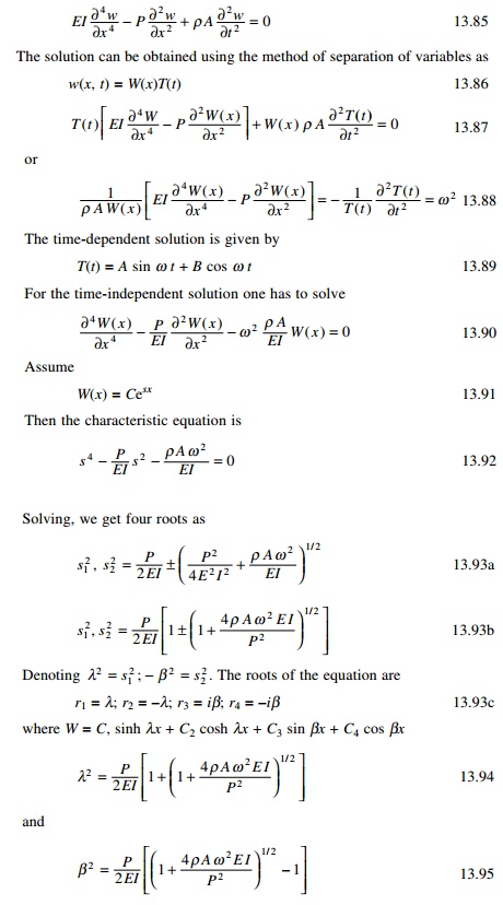
The natural frequency expressed in Eq. 13.105 extends the application to single span beams with different boundary conditions by selecting appropriate value for β from Table 13.3. If EI = 0 the problem degenerates to that of a flexible taut cable discussed in Section 13.1. As we see from Eq. 13.105 the tensile load ‘stiffens’ the beam, thereby increasing the natural frequency.

1  Beams subjected to axial compression

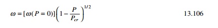
In the above equation substitute �'P for P to get the frequency for a beam subjected to axial compression:

The following observations can be made:

•       If P = 0 the natural frequency will be the same as that of a simply supported beam.

•       If EI = 0 the frequency reduces to that of a string.

•       If P > 0 the natural frequency increases with tensile force as it stiffens the beams.

•       If P < 0 the natural frequency decreases with compressive force and approaches zero when P = P_cr.

Effect of rotary inertia and shear deformation

If the cross-sectional dimensions are not small compared with the length of the beam, we need to consider the effects of rotary inertia and shear deformation. This was first presented by Timoshenko and is known as thick beam theory or Timoshenko beam theory.

If the effect of shear deformation is disregarded (see Fig. 13.13), the tangent to the deflection centre line OT coincides with the normal to the face B′C′ (since the cross-section normal to the centre line remains normal even after deformation). Owing to deformation, the tangent to the deformed centre line O′T will not be perpendicular to B′C′.

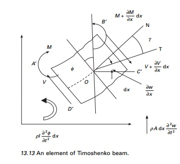
The angle between tangent to the deformed line OT and normal to the face ON denotes the shear deflection of an element. Since positive shear on the fight face B′C′ acts downward we have from Fig. 13.13

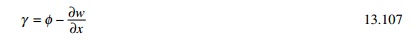
where φ denotes the slope of the deflection curve due to bending deflection alone. Note that because of shear alone, the element distorts and does not rotate.

The bending moment M and the shear force V are related to the slope and deflection as

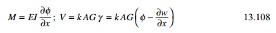
where G denotes the modulus of rigidity of the material of the beam and ‘k’ is a constant known as Timoshenko’s shear coefficient which depends on the shape of the cross section. For a rectangular section k = 5/6; circle = 9/10. The equation of motion can be derived as follows.

1.       For translation in the Z direction

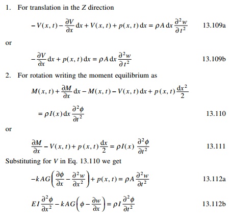
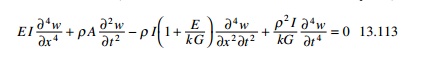
By solving Eq. 13.112a for ∂φ/∂x and substituting the result of Eq. 13.112a in Eq. 112b we obtain (for uniform beams and for free vibration p = 0)

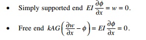
For most practical situations, the increased accuracy obtained by including shear and rotary effect is much less than the modelling errors. The contribution for shear stress is generally less than the contribution for rotation, but both effects can generally be ignored for shallow beams. The following boundary conditions are to be applied.

Fixed end φ = w = 0.

Example 13.7

Determine the effects of rotary inertia and shear deflection on the natural frequency of a simply supported uniform beam.

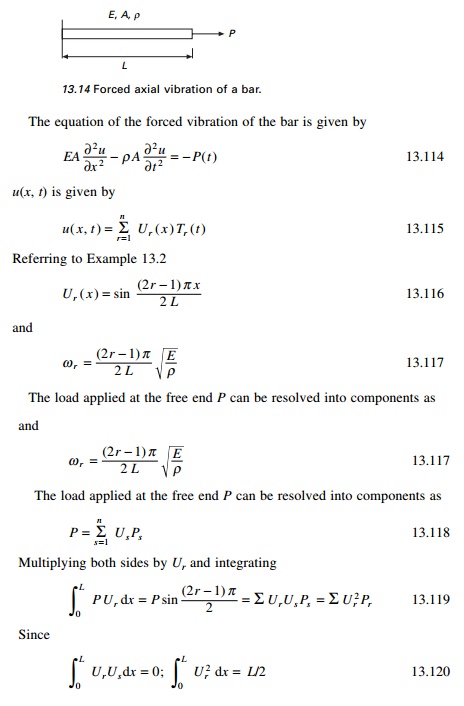
Forced axial vibration of bars

Consider a bar as shown in Fig. 13.14 which is fixed at one end and free at the other end to which an exciting force P(t) is applied.

A suddenly applied load therefore produces twice the deflection than that one would obtain if the load is applied gradually.

Example 13.8

Forced vibration of a flexural member

The simply supported beam shown in Fig. 13.15a having mass density ρ and cross-sectional area A, moment of inertia I has a distributed load whose variation with time is shown in Fig. 13.15b. Determine the expression for dynamic deflection of the beam.

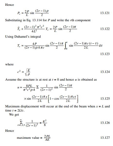
Example 13.9

A simply supported beam carries a uniformly distributed load of q. Find the resulting vibration of the beam when the load is suddenly removed.

Beams subjected to moving loads

A particular class of problem which has long been of interest to engineers involves the determination of the dynamic response of a beam or girder resulting from the passage of a force or mass across the span. Examples include the analysis of crane beams and moving vehicles in highway and railway bridges.

1 Constant force with constant velocity

Let us consider a constant force F moving across the span of the beam at constant velocity v as indicated in Fig. 13.16. The dynamic deflection may be represented by the summation of modal components as

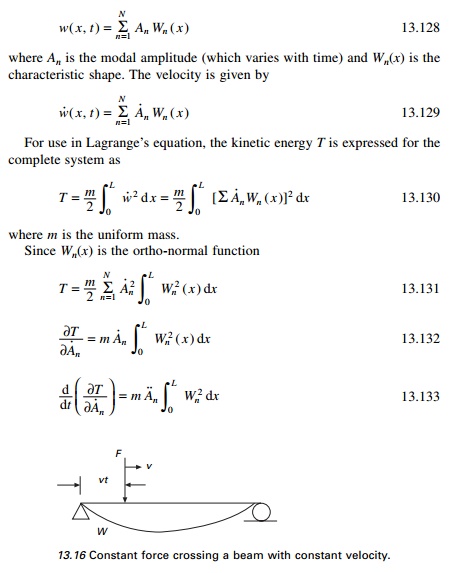
where A_n is the modal amplitude (which varies with time) and W_n(x) is the characteristic shape. The velocity is given by

For use in Lagrange’s equation, the kinetic energy T is expressed for the complete system as

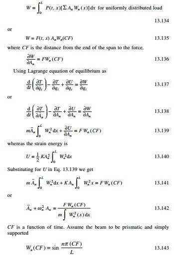
The work done by external dynamic force during an arbitrary distortion is

where CF is the distance from the end of the span to the force.

Using Lagrange equation of equilibrium as

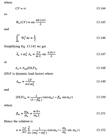
CF is a function of time. Assume the beam to be prismatic and simply supported

Example 13.10

Derive the mid-span deflection of a simple beam traversed by a constant force, ignoring damping and including only a fundamental mode (higher modes are of negligible importance). The parameters of the system are given as M = 2 kg; EI = 78 700 N m², L = 10 m, v = 12.5 m/s. Calculate the critical speed to cause resonance.

The first term of the above expression is forced and the second one is free vibration. The deflection is plotted in Fig. 13.17 as a fraction of mid-span deflection. The abscissa may be considered to be either time or the position of load on the span. Plotted separately is the forced part of the solution which is very nearly equal to the static deflection ordinates of Fig. 13.17 may also be regarded as the ratio of dynamic to static moments.

Summary

The dynamic analysis of string, bar and beam with distributed properties (mass and elasticity) and subjected to various types of loading were presented in this chapter. The extension of the analysis to multi-span continuous beams, though possible, is complex and impractical. The results obtained from these single span beams are particularly important in evaluating an approximate method based on discrete models.