Summary

SUMMARY

• A random variable X is a function defined on a sample space S into the real numbersℝ  such that the inverse image of points or subset or interval of ℝ is an event in S, for which probability is assigned.

• A random variable X is defined on a sample space S into the real numbers ℝ is called discrete random variable if the range of X is countable, that is, it can assume only a finite or countably infinite number of values, where every value in the set S has positive probability with total one.

• If X is a discrete random variable with discrete values x₁, x₂, x₃,... x_n..., then the function denoted by f(.) or p(.) and defined by f(x_k) = P(X = x_k) for k = 1,2,3,...n,... is called the probability mass function of X

• The function f(x) is a probability mass function if

(i) f(x_k) ≥ 0 for k = 1,2,3,...n,... and (ii) ∑_k f (x_k ) = 1

• The cumulative distribution function F(x) of a discrete random variable X, taking the values x₁, x₂, x₃,... such that x₁ < x₂ < x₃ < ^… with probability mass function f(x_i) is

F (x) = P(X ≤ x) = ∑_xi≤x f (x_i ), x ∈ ℝ

• Suppose X is a discrete random variable taking the values x₁, x₂, x₃,... such that x₁ < x₂ < x₃,... and F(x_i) is the distribution function. Then the probability mass function f(x_i) is given by f(x_i) = F(x_i) – F(x_i–1), i = 1,2,3, ...

• Let S be a sample space and let a random variable X : S → ℝ that takes any value in a set I of ℝ. Then X is called a continuous random variable if P(X = x) = 0 for every x in I.

• A non-negative real valued function f(x) is said to be a probability density function if, for each possible outcome x, x ∈ [a,b] of a continuous random variable X having the property.

P(a ≤ x ≤ b) = ^b∫_a f (x) dx

• Suppose F(x) is the distribution function of a continuous random variable X. Then the

probability density function f(x) is given by

 f(x) = dF(x) / dx = F′(x) , whenever derivative exists.

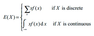
• Suppose X is a random variable with probability mass or density function f(x) The expected value or mean or mathematical expectation of X, denoted by E(x) or μ is

• The variance of the random variable X denoted by V(X) or σ² (or σ_x²) is

V(X) = E(X – E(X))² = E(X – μ)²

Properties of Mathematical expectation and variance

(i) E(aX + b) = aE(X) + b,

where a and b are constants

Corollary 1: E(aX) = aE(X)

  ( when b = 0)

Corollary 2: E(b) = b

(when a = 0)

(ii) Var(X) = E(X²) – (E(X))²

(iii) Var(aX + b) = a²Var(X) where a and b are constants

Corollary 3: V(aX ) = a²V(X) (when b = 0)

Corollary 4: V(b) = 0 (when a = 0)

• Let X be a random variable associated with a Bernoulli trial by defining it as X (success) = 1 and X (failure) = 0, such that

• X is called a Bernoulli random variable and f(x) is called the Bernoulli distribution.

• If X is a Bernoulli’s random variable which follows Bernoulli distribution with parameter p, the mean μ and variance σ ² are

 μ=p and  σ² = pq

• A discrete random variable X is called binomial random variable, if X is the number of successes in n-repeated trials such that

(i) The n- repeated trials are independent and n is finite

(ii) Each trial results only two possible outcomes, labelled as ‘success’ or ‘failure’

(iii) The probability of a success in each trial, denoted as p, remains constant

• The binomial random variable X equals the number of successes with probability p for a success and q = 1 – p for a failure in n-independent trials, has a binomial distribution denoted by X ~ B(n, p). The probability mass function of X is f (x) =  p^x (1 − p)^{n− x} , x = 0,1, 2,..., n.

• If X is a binomial random variable which follows binomial distribution with parameters p and n, the mean μ and variance σ² are μ = np and σ² = np(1 – p).