Probability Distributions | Mathematics - Types of Random Variable | 12th Maths : UNIT 11 : Probability Distributions
Chapter: 12th Maths : UNIT 11 : Probability Distributions
Types of Random Variable
Types of Random
Variable
In this
chapter we shall restrict our study to two types of random variables, one is a
random variable assuming at most a countable number of values and another is a
random variable assuming the values continuously. That is
(i) Discrete
Random variable (for counting the quantity)
(ii) Continuous
Random variable (for measuring the quantity)
1. Discrete random variables
In this
section we discuss
(i) Discrete
random variables
(ii) Probability
mass function
(iii) Cumulative
distribution function.
(iv) Obtaining
cumulative distribution function from probability mass function.
(v) Obtaining
probability mass function from cumulative distribution function.
If the
range set of the random variables is discrete set of numbers then the inverse
image of random variable is either finite or countably infinite. Such a random
variable is called discrete random variable. A random variable defined on a
discrete sample space is discrete.
Definition 11.2 (Discrete Random Variable)
A random variable X is
defined on a sample space S into the
real numbers is called discrete random variable if the range of X is countable, that is, it can assume
only a finite or countably infinite number of values, where every value in the
set S has positive probability with
total one.
Remark
It is
also possible to define a discrete random variable on continuous sample space.
For instance,
(i) for
a continuous sample space S =
[0,1] , the random variable defined by X
(ω) = 10 for all ω ∈ S, is a discrete random variable.
(ii) for
a continuous sample space S =
[0, 20] , the random variable defined by
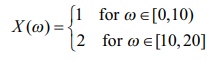
is a
discrete random variable.
2. Probability Mass Function
The
probability that a discrete random variable X
takes on a particular value x, that
is P
( X = x) , is frequently denoted by f (
x) or p ( x) . The
function f ( x) is typically called the probability mass function, although some
authors also refer to it as the probability function or the frequency function.
In this chapter, when the random variable is discrete, the common terminology
the probability mass function is used and its common abbreviation is pmf.
Definition 11.3 (Probability mass function)
If X is a discrete
random variable with discrete values
x1 , x2 , x3 , xn
, then the
function denoted by f (.) or p(.) and defined by
f ( xk ) = P ( X= xk ), for k =1, 2, 3,
n,
is called the probability mass function of X
Theorem 11.1 (Without proof)
The function f ( x) is a probability mass function if and
only if it satisfies the following properties for the set of real values x1, x2, x3, ... xn ....
(i) f (xk) ≥ 0 for k
=1, 2, 3, n,
and
(ii) ∑k f (xk) =1
Note:
(i) The
set of probabilities { f (xk ) = P ( X = xk ),
k = 1, 2, 3,. . . . n , . . . } is also known as probability distribution of discrete random variable
(ii) Since
the random variable is a function, it can be presented
(a) in
tabular form (b) in graphical form and (c) in an expression form
Example 11.5
Two fair
coins are tossed simultaneously (equivalent to a fair coin is tossed twice).
Find the probability mass function for number of heads occurred.
Solution
The
sample space S =
{ H , T} × {H , T}
That is S = { TT , TH, HT , HH
}
Let X be the random variable denoting the
number of heads.
Therefore
X (TT) =0,
X (TH) =1,
X (HT) = 1, and
X (HH) =2.
Then the
random variable X takes on the values
0, 1 and 2

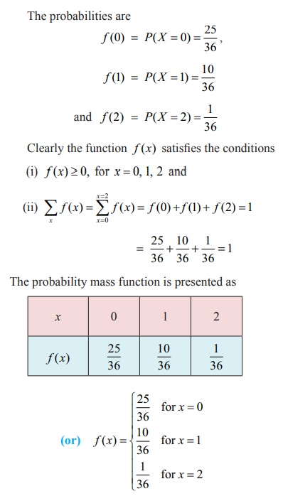
The
probabilities are given by
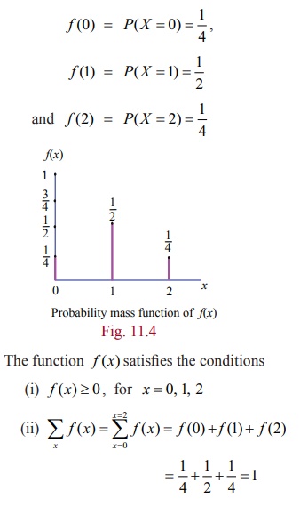
Therefore
f ( x) is a probability mass function.
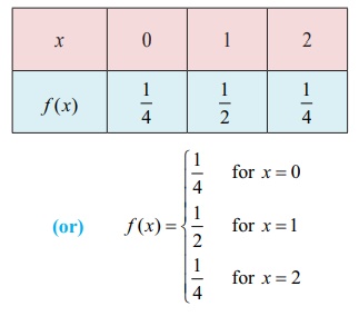
The
probability mass function is given by
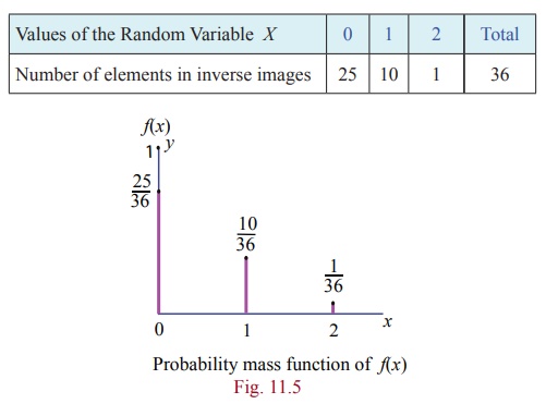
Example 11.6
A pair
of fair dice is rolled once. Find the probability mass function to get the
number of fours.
Solution
Let X be a random variable whose values x are the number of fours.
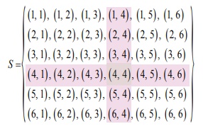
The
sample space S is given in the table.
It can
also be written as
S = {(i, j)} , where i = 1, 2, 3,. . .6 and j
= 1, 2, 3, 6
Therefore
X takes on the values of 0, 1, and 2.
We
observe that
(i) X = 0, if (i , j) for
i ≠ 4, j ≠ 4,
(ii) X = 1, if (1,4) , (2,4) , (3,4)
, (5,4) , (6,4) , (4,1) , (4, 2) , (4, 3) , (4, 5) , (4, 6)
(iii) X = 2, if (4, 4) ,
Therefore,
3. Cumulative Distribution Function or Distribution Function
There are many situations to compute the probability that the observed value of a random variable X will be less than or equal to some real number x . Writing F( x) = P (X≤ x) for every real number x , we call F ( x) , the cumulative distribution function or distribution function of the random variable X and its common abbreviation is cdf .
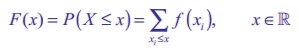
Definition 11.4: (cumulative distribution function)
The cumulative
distribution function F (
x) of a discrete random
variable X
, taking the values x1
, x2
, x3
, such that
x1 < x2 < x3 < … with probability mass function f (xi) is
F ( x) = P ( X ≤ x ) = ∑xi≤x f ( xi ),
x ∈ ℝ
The
distribution function of a discrete random variable is known as Discrete
Distribution Function. Although, the probability mass function f ( x)
is defined only for a set of discrete
values x1, x2 , x3 , . . . , the cumulative distribution function F ( x)
is defined for all real values of x ∈ ℝ.
We can
compute the cumulative distribution function using the probability mass function
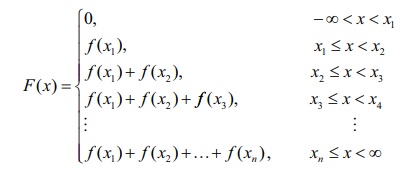
If X takes only a finite number of values x1 , x2 , x3
, . . . xn , where x1 < x2 < x3 <,
. . . < xn , then
the cumulative distribution function is given by
For a
discrete random variable X, the
cumulative distribution function satisfies the following properties.
(i) 0 ≤
F (x) ≤ 1 , for all x ∈ ℝ.
(ii) F ( x)
is real valued non-decreasing function { x
< y, then F ( x) ≤ F (
y) .
(iii) F ( x)
is right continuous function (limx→a+
F(x) = F (a) .
(iv) lim
x → -∞ F (x) = F(-∞)
= 0 .
(v) lim
x → +∞ F (x) = F(+∞) = 1 .
(vi) P (x1 < X ≤ x2 ) = F (x2) − F (x1).
(vii) P (X
> x) = 1 − P (X≤ x) = 1 − F (x) .
(viii) P ( X = xk ) = F( xk ) − F( xk− ) .
Note
Some
authors use left continuity in the definition of a cumulative distribution
function F ( x) , instead of right continuity.
4. Cumulative Distribution Function from Probability Mass function
Both the
probability mass function and the cumulative distribution function of a
discrete random variable X contain
all the probabilistic information of X.
The probability distribution of X is determined by either of them. In
fact, the distribution function F of
a discrete random variable X can be
expressed in terms of the probability mass function f(x) of X and vice versa.
Example 11.7
If the
probability mass function f ( x) of a random variable X is
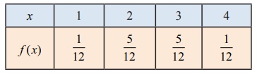
find (i)
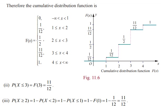
its cumulative distribution function, hence find (ii) P( X ≤
3) and, (iii) P( X ≥ 2)
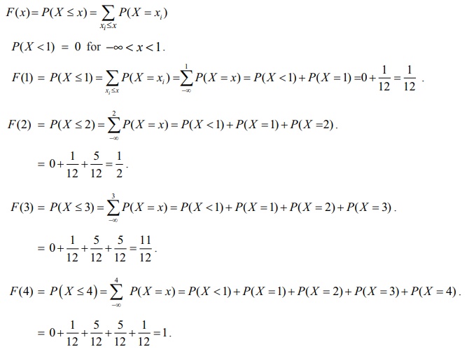
Solution
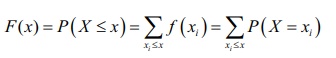
(i) By
definition the cumulative distribution function for discrete random variable is
F ( x) = P(
X≤ x) = ∑xi≤xP( X = xi )
Therefore
the cumulative distribution function is
Example 11.8
A six
sided die is marked ‘1’ on one face, ‘2’ on two of its faces, and ‘3’ on
remaining three faces. The die is rolled twice. If X denotes the total score in two throws.
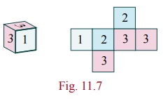
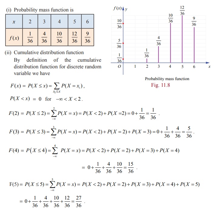
(i) Find
the probability mass function.
(ii) Find
the cumulative distribution function.
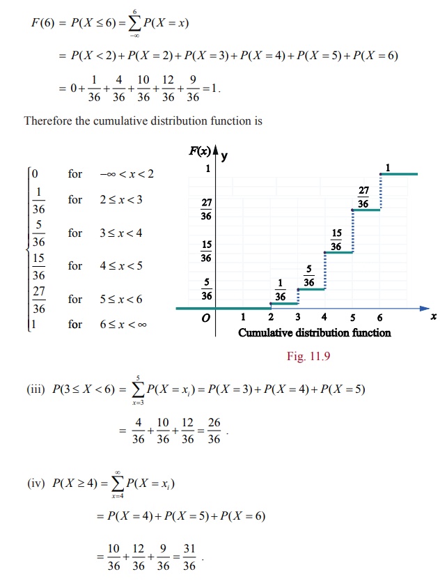
(iii) Find
P (3≤ X < 6) (iv) Find P ( X ≥ 4) .
Solution:
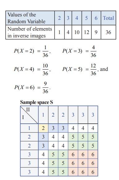
Since X denotes the total score in two throws,
it takes on the values 2, 3, 4, 5, and 6.
From the
Sample space S, we have
5. Probability Mass Function from Cumulative Distribution Function
For a
discrete random variable X, the
cumulative distribution function F has
jumps at each of the xi , and is constant between
successive xi ′s . The height of the jump at xi f( xi
) ; in this way the is probability at xi
can be retrieved from F .
Suppose X is a discrete random
variable taking the values x1 , x2 , x3 , such that x1 < x2 , < x3 and F ( xi ) is the distribution function. Then the probability mass
function f ( xi ) is given by
f (xi) = F (xi ) F (xi-1 )
, i = 1, 2, 3, . . .
Note
The jump
of a function F ( x) at x = a is |F
( a +
) −
F ( a − )|. Since F is non-decreasing and continuous to
the right, the jump of a cumulative distribution function F is P( X = x) = F( x) − F( x−
) .
Here the
jump (because of discontinuity) acts as a probability. That is, the set of
discontinuities of a cumulative distribution function is at most countable!
Example 11.9
Find the
probability mass function f ( x) of the discrete random variable X whose cumulative distribution function
F ( x) is given by
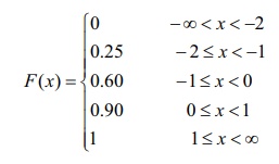
Also
find (i) P( X < 0) and (ii) P( X ≥ − 1) .
Solution
Since X is a discrete random variable, from
the given data, X takes on the values
−2, −1,
0, and 1.
For
discrete random variable X, by
definition, we have f ( x) = P(
X = x)
Therefore
left hand limit of F(x) at x = −2 is F ( −2
−
)
f(−2) = P(X = −
2) = F(− 2) − F(− 2
− ) = 0.25 − 0 = 0.25.
Similarly
for other jump points, we have
f (−1) = P(X = −
1) = F(− 1) − F(−2) = 0.60 − 0.25 = 0.35.
f (0) = P(X = 0) = F(0) − F(−1) = 0.90 − 0.60 = 0.30 ,
f (1) = P( X = 1) = F(1) − F(0) = 1 − 0.90 = 0.10 .
Therefore
the probability mass function is
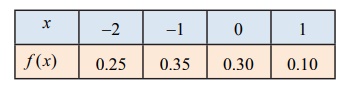
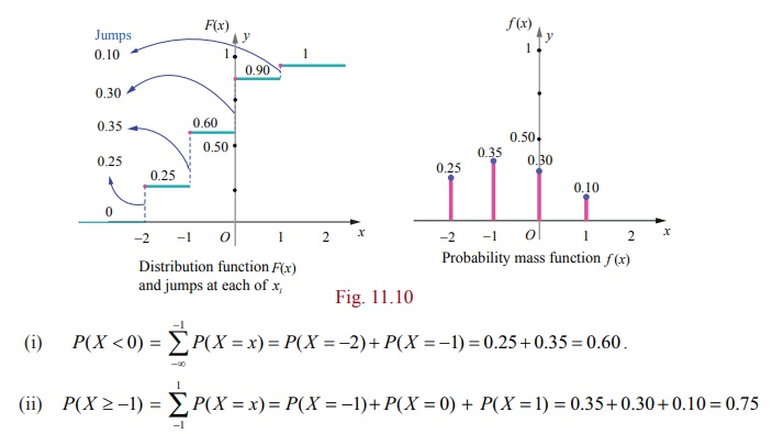
The
distribution function F ( x) has jumps at x = − 2, − 1, 0, and 1. The jumps are respectively 0.25, 0.35,
0.30, and 0.1 is shown in the figure given below.
These
jumps determine the probability mass function
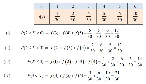
Example 11.10
A random
variable X has the following
probability mass function.
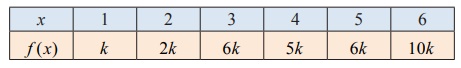
Find (i)
P (2 < X < 6) (ii) P (2 ≤ X < 5) (iii) P(X
≤ 4) (iv) P(3< X)
Solution
Since
the given function is a probability mass function, the total probability is one.
That is ∑x f (x) = 1.
From the
given data k + 2k + 6k + 5k + 6k
+ 10k = 1
30k =
1
⇒
k = 1/30
Therefore
the probability mass function is
Related Topics