Definition, Properties | Probability Distributions | Mathematics - Continuous Distributions | 12th Maths : UNIT 11 : Probability Distributions
Chapter: 12th Maths : UNIT 11 : Probability Distributions
Continuous Distributions
Continuous
Distributions
In this
section we learn
(i) Continuous
random variable
(ii) Probability
density function
(iii) Distribution
function (Cumulative distribution function).
(iv) To
determine distribution function from probability density function.
(v) To
determine probability density function from distribution function.
Sometimes
a measurement such as current in a copper wire or length of lifetime of an
electric bulb, can assume any value in an interval of real numbers. Then any
precision in the measurement is possible. The random variable that represents
this measurement is said to be a continuous random variable. The range of the
random variable includes all values in an interval of real numbers; that is,
the range can be thought of as a continuum of real numbers
1. The definition of continuous random variable
Definition 11.5 (Continuous Random Variable)
Let S be a sample space and
let a random variable X : S → ℝ that takes on any value in a set I of ℝ . Then X is called a continuous random variable if P (X = x) = 0 for every x in I
2. Probability density function
Definition 11.6: (Probability density function)
A non-negative real
valued function f ( x) is said to be a probability density
function if, for each possible
outcome x, x ∈ [a,b] of a continuous random
variable X having the property
Theorem 11.2 (Without proof)
A function f (.) is a probability
density function for some continuous random variable X if and only if it satisfies the following properties.
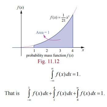
(i) f (x)
≥ 0 , for every x and (ii) ∞∫-∞f (x)dx = 1 .
Note
It
follows from the above definition, if X
is a continuous random variable,
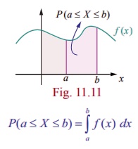
P(a ≤ X ≤ b) = b∫a f( x) dx,
which means that P( X = a) = a∫a f (x) dx = 0
That is
probability when X
takes on any one particular value is zero.
3. Distribution function (Cumulative distribution function)
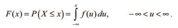
Definition 11.7 : (Cumulative Distribution Function)
The distribution function or cumulative distribution function F ( x) of a continuous random variable X with
probability density f(x) is
Remark
(1) In
the discrete case, f (a) = P (X = a) is the probability that X takes the value a.
In the
continuous case, f (x) at x = a is not the
probability that X takes the value a, that is f (a) ≠ P (X
= a) . If X is continuous type, P (X
= a) = 0 for a ∈ ℝ.
(2) When
the random variable is continuous, the summation used in discrete is replaced
by integration.
(3) For
continuous random variable
P(a < X < b) = P(a ≤ X
< b) = P(a < X ≤ b) = P(a ≤ X ≤ b)
(4) The
distribution function of a continuous random variable is known as Continuous
Distribution Function.
Properties of distribution function
For a
continuous random variable X, the cumulative distribution function satisfies
the following properties.
(i) 0 ≤
F ( x) ≤ 1 .
(ii) F (
x) is a real valued
non-decreasing. That is, if x < y , then F ( x) ≤ F (
y) .
(iii) F (
x) is continuous everywhere.
(iv) lim
x → −∞ F (x) = F(
− ∞) = 0 and lim x → ∞ F (x) = F
(+∞) = 1.
(v) P (X
> x) = 1 − P (X≤
x) = 1 − F (x) .
(vi) P(a < X < b) = F(b)
−F(a) .
Example 11.11
Find the constant C
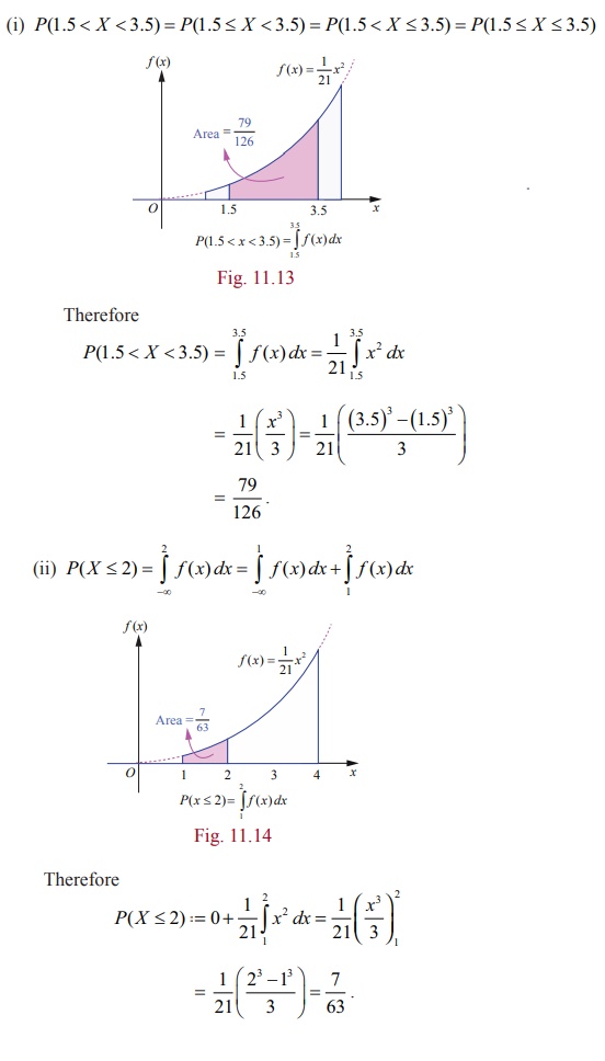
such that the function 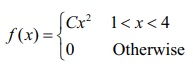 is a density function, and compute (i) P(1.5 < X
<
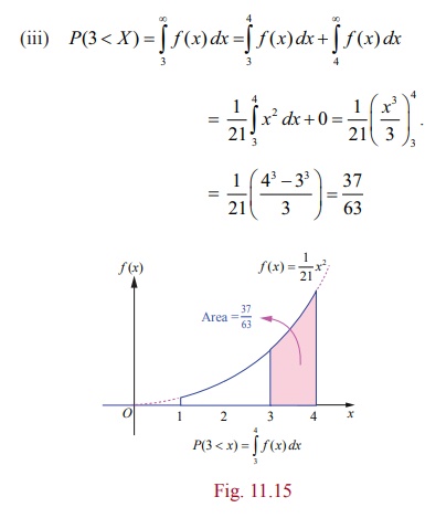
3.5) (ii) P ( X ≤ 2) (iii) P(3 <
X ) .
is a density function, and compute (i) P(1.5 < X
<
3.5) (ii) P ( X ≤ 2) (iii) P(3 <
X ) .
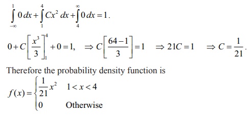
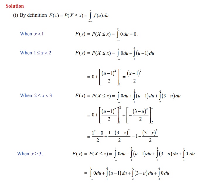
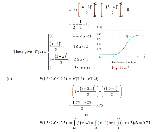
Solution
Since the given function is a probability density function,
From the given information,
Since f ( x) is continuous, the probability that X is equal to any particular value is
zero.
Therefore when the random variable is continuous, either or
both of the signs < by ≤ and > by ≥
can be interchanged. Thus
4. Distribution function from Probability density function
Both the probability density function and the cumulative
distribution function (or distribution function) of a continuous random
variable X contain all the
probabilistic information of X . The probability distribution of X is determined by either of them. Let
us learn the method to determine the
distribution function F of a
continuous random variable X from the
probability density function f (x)
of X and vice versa.
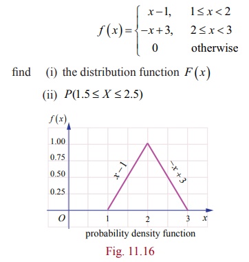
Example 11.12
If X is the random
variable with probability density function f(x) given by,
Check:
(i) Whether F ( x) is continuous everywhere.
(ii) From the Fig. 11.16, triangle area =
1/2 bh = 1.
5. Probability density function from Probability distribution function.
Let us learn the method to determine the probability density
function f ( x) from the distribution function F ( x) of a continuous
random variable X .
Suppose F ( x) is the distribution function of a continuous random variable X . Then the probability
density function f(x) is given by
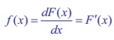
f( x) = dF(x) / dx = F ′ ( x) , wherever derivative exists.
Example 11.13
If X
is the random variable with distribution function F (x) given by,
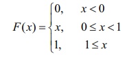
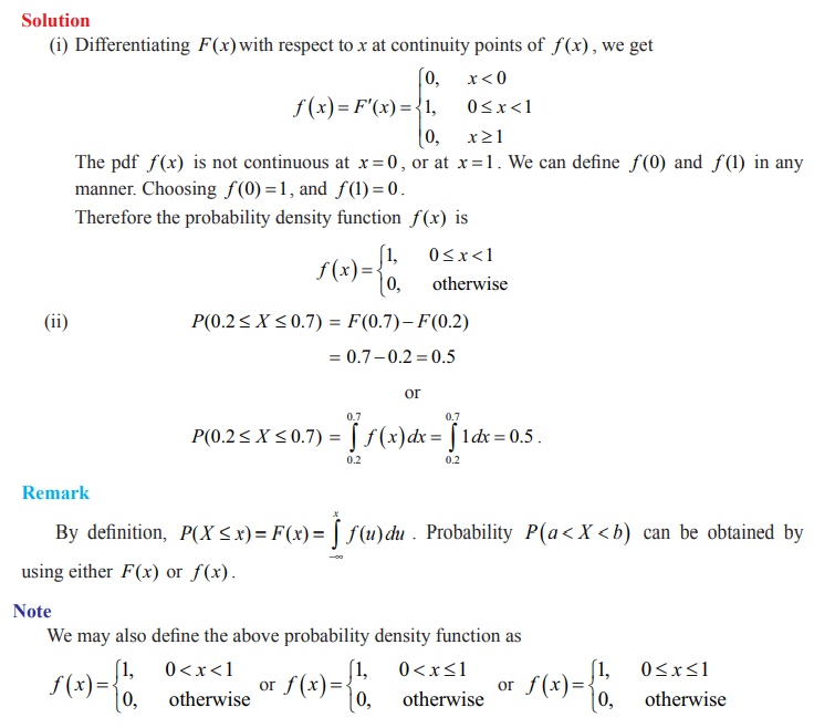
then find (i) the probability density function f (x)
(ii) P ( 0.2 ≤ X 0.7).
Solution
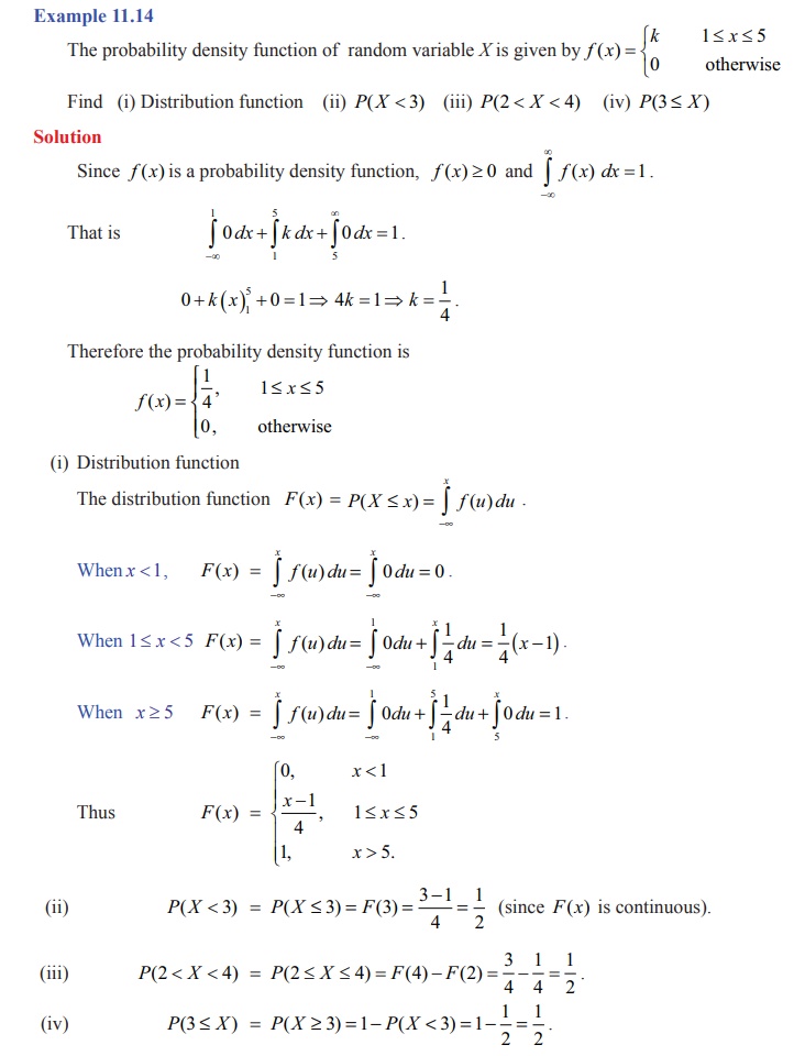
Example 11.15
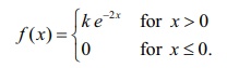
Let X
be a random variable denoting the life time of an electrical equipment having
probability density function
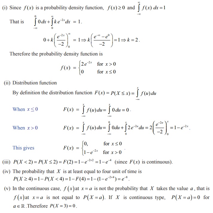
Find (i) the value of k (ii) Distribution function (iii) P (X< 2)
(iv) calculate the probability that X is at least for four unit of time (v)
P (X = 3) .
Solution
Related Topics