Theoretical Distributions: Some Special Discrete Distributions

Theoretical Distributions: Some Special Discrete Distributions

In the previous section we have dealt with various general probability distributions with mean and variance. We shall now learn some discrete probability distributions of special importance.

In this section we learn the following discrete distributions.

(i) The One point distribution

(ii) The Two point distribution

(iii) The Bernoulli distribution

(iv) The Binomial distribution.

(i) The One point distribution

The random variable X has a one point distribution if there exists a point x₀ such that, the probability mass function f ( x) is defined as f (x) = P ( X = x₀ ) = 1 .

That is the probability mass is concentrated at one point.

The cumulative distribution function is

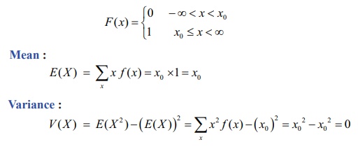
Therefore the mean and the variance are respectively x₀ and 0 .

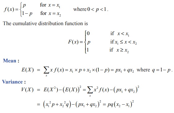
(ii) The Two point distribution

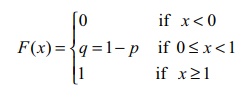
(a) Unsymmetrical Case: The random variable X has a two point distribution if there exists two values x₁ and x₂ , such that

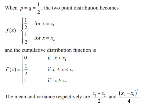
(b) Symmetrical Case:

(iii) The Bernoulli distribution

Independent trials having constant probability of success p were first studied by the Swiss mathematician Jacques Bernoulli (1654–1705). In his book The Art of Conjecturing, published by his nephew Nicholas eight years after his death in 1713, Bernoulli showed that if the number of such trials were large, then the proportion of them that were successes would be close to p.

In probability theory, the Bernoulli distribution, named after Swiss mathematician Jacob Bernoulli is the discrete probability distribution of a random variable. A Bernoulli experiment is a random experiment, where the outcomes is classified in one of two mutually exclusive and exhaustive ways, say success or failure (example: heads or tails, defective item or good item, life or death or many other possible pairs). A sequence of Bernoulli trails occurs when a Bernoulli experiment is performed several independent times so that the probability of success remains the same from trial to trial. Any nontrivial experiment can be dichotomized to yield Bernoulli model.

Definition 11.10: ( Bernoulli’s distribution)

Let X be a random variable associated with a Bernoulli trial by defining it as

X (success) = 1 and X (failure) = 0, such that

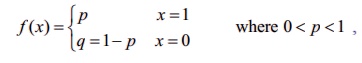
then X is called a Bernoulli random variable and f ( x) is called the Bernoulli distribution.

Or equivalently

If a random variable X is following a Bernoulli’s distribution, with probability p of success can be denoted as X ~ Ber( p) , where p is called the parameter, then the probability mass function of X is

 f (x) = p^x (1 − p)^1−x , x = 0, 1

The cumulative distribution of Bernoulli’s distribution is

Mean :

 E ( X ) = ∑_xx f (x) = 1×  p + 0 ×  (1 − p ) = p ,

Note that, since X takes only the values 0 and 1, its expected value p is “never seen”.

Variance :

 V ( X ) = E ( X² ) – (E ( X ))² = ∑ x² f (x ) p²

  = ( 1²p + 0²q) – p² = p(1 – p ) = pq            where q = 1 – p

If X is a Bernoulli’s random variable which follows Bernoulli distribution with parameter p, the mean μ and variance σ ² are

 μ = p and σ² = pq

When p = q = 1/2 , the Bernoulli’s distribution become

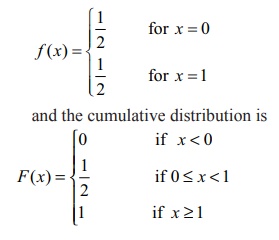
The mean and variance are respectively are 1/2 and ¼. 

(iv) The Binomial Distribution

The Binomial Distribution is an important distribution which applies in some cases for repeated independent trials where there are only two possible outcomes: heads or tails, success or failure, defective item or good item, or many other such possible pairs. The probability of each outcome can be calculated using the multiplication rule, perhaps with a tree diagram.

Suppose a coin is tossed once. Let X denote the number of heads. Then X ~ Ber( p), because we get either head (X = 1) or tail (X = 0) with probability p or 1 − p.

Suppose a coin is tossed  n times. Let X denote the number of heads. Then X takes on the values 0, 1, 2, …, n. The probability for getting x number of heads is given by

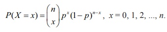
X = x , corresponds to the combination of x heads in n tosses, that is  ways of heads and remaining n − x tails. Hence, the probability for each of thos e outcomes is equal to p ^x (1 − p)^n−x .

Binomial theorem is suitable to apply when n is small number less than 30.

Definition 11.11: Binomial random variable

A discrete random variable X is called binomial random variable, if X is the number of successes in n -repeated trials such that

(i) the n- repeated trials are independent and n is finite

(ii) each trial results only two possible outcomes, labelled as ‘success’ or ‘failure’

(iii) the probability of a success in each trial, denoted as p, remains constant.

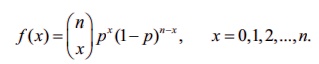
Definition 11.12 : Binomial distribution

The binomial random variable X equals the number of successes with probability p for a success and q = 1 − p for a failure in n-independent trials, has a binomial distribution denoted by X ~ B(n, p). The probability mass function of X is

The name of the distribution is obtained from the binomial expansion. For constants a and b, the binomial expansion is

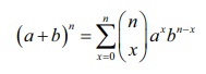
Let p denote the probability of success on a single trial. Then, by using the binomial expansion with a = p and b = 1 − p , we see that the sum of the probabilities for a binomial random variable is 1. Since each trial in the experiment is classified into two outcomes, {success, failure}, the distribution is called a “bi’’-nomial.

If X is a binomial random variable which follows binomial distribution with parameters p and n, the mean μ and variance σ ² are

 μ = np and σ² = np(1 − p)

The expected value is in general not a typical value that the random variable can take on. It is often helpful to interpret the expected value of a random variable as the long-run average value of the variable over many independent repetitions of an experiment. The shape of a binomial distribution is symmetrical when p = 0.5 or when n is large.

When p = q = 1/2, , the binomial distribution becomes

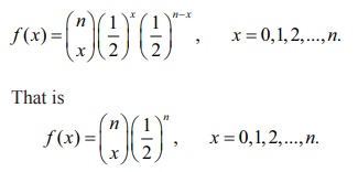
The mean and variance are respectively are n/2 and n/4.

Example 11.19

Find the binomial distribution for each of the following.

(i) Five fair coins are tossed once and X denotes the number of heads.

(ii) A fair die is rolled 10 times and X denotes the number of times 4 appeared.

Solution

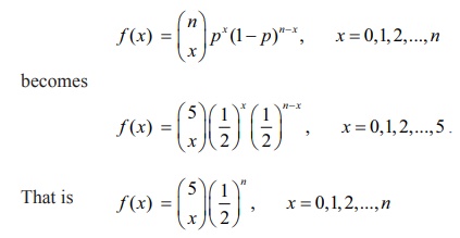
(i) Given that five fair coins are tossed once. Since the coins are fair coins the probability of getting an head in a single coin is p = 1/2 and q = 1 − p = 1/2

Let X denote the number of heads that appear in five coins. X is a binomial random variable that takes on the values 0, 1,2,3,4 and 5, with n = 5 and p = 1/2.That is X ~ B(5, ½).

Therefore the binomial distribution is

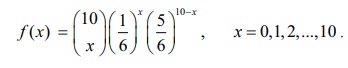
(ii) A fair die is rolled ten times and X denotes the number of times 4 appeared. X is binomial random variable that takes on the values 0, 1, 2, 3, 10 , with n = 10 and p = 1/6. That is X ~ B(10, 1/6).

Probability of getting a four in a die is p = 1/6 and q = 1 − p = 5/6.

Therefore the binomial distribution is

Example 11.20

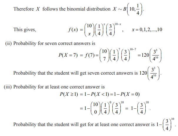
A multiple choice examination has ten questions, each question has four distractors with exactly one correct answer. Suppose a student answers by guessing and if X denotes the number of correct answers, find (i) binomial distribution (ii) probability that the student will get seven correct answers (iii) the probability of getting at least one correct answer.

Solution

(i) Since X denotes the number of success, X can take the values 0,1, 2 ,.. .,10

The probability for success is p = 1/4 and for failure q = 1 – p = 3/4 and n=10.

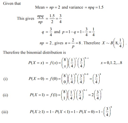
Example 11.22

The mean and variance of a binomial variate X are respectively 2 and 1.5. Find

 (i) P (X = 0 ) (ii) P (X=1) (iii) P (X≥1)

Solution

To find the probabilities, the values of the parameters n and p must be known.

Given that

 Mean = np = 2 and variance = npq = 1 5.

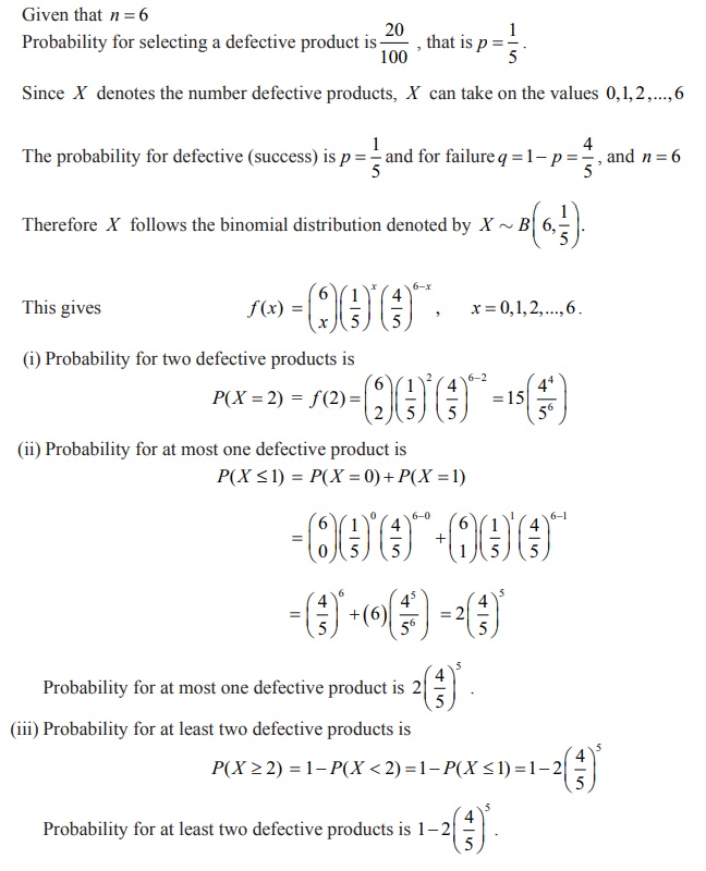
Example 11.22

On the average, 20% of the products manufactured by ABC Company are found to be defective. If we select 6 of these products at random and X denotes the number of defective products find the probability that (i) two products are defective (ii) at most one product is defective (iii) at least two products are defective.

Solution