Mathematics - Partial Derivatives | 12th Maths : UNIT 8 : Differentials and Partial Derivatives
Chapter: 12th Maths : UNIT 8 : Differentials and Partial Derivatives
Partial Derivatives
Partial
Derivatives
In this
section, we shall see how the concept of derivative for functions of one
variable may be generalized to real-valued function of several variables. First
we consider functions of two variables.
Let A = { ( x, y ) | a
<
x < b,
c < y
<
d } ŌŖé ŌäØ2 , and F : A ŌåÆ
ŌäØ be a real-valued function. Suppose
that (x0 ,
y0 ) Ōłł A ; and we are interested in finding
the rate of change of F at (
x0 , y0 ) with respect to the change only in the variable x .
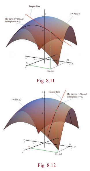
As we have seen above F ( x, y0
) is a function of x alone and it
will represent a curve obtained by intersecting the surface z = F
( x , y) with y =
y0 plane. So we can
discuss the slope of the tangent to the curve z = F ( x , y0
) at x = x0
by finding derivative of F ( x, y0
) with respect to x and evaluating it
at x = x0
. Similarly, we can find the slope of the curve z = F ( x0 , y) at y =
y0 by finding derivative
of F ( x0 , y) with
respect to y and evaluating it at y = y0
. These are the key ideas that motivate us to define partial derivatives below.
Definition 8.8
Let A = {( x, y )| a
<
x < b,
c < y
<
d } ŌŖé ŌäØ2 , F : A ŌåÆ
and ( x0 , y0 ) Ōłł A
(i) We
say that F has a partial derivative
with respect to x at ( x0 , y0 ) Ōłł
A if

exists.
In this case, the limit value is denoted by ŌłéF/Ōłéx ( x0 , y0 ) .
(ii) We
say F has a partial derivative with respect to y at ( x0 , y0 ) Ōłł A if

exists.
In this case, the limit value is denoted by ŌłéF/Ōłéy ( x0 , y0 ) .
Remarks
1. Partial
derivatives for functions of three or more variables are defined exactly in a
similar manner.
2. We
read ŌłéF as ŌĆ£partial F
ŌĆØ and Ōłéx as ŌĆ£partial
x ŌĆØ. And we read ŌłéF/Ōłéx as ŌĆ£partial F by partial
x ŌĆØ. It is also read as ŌĆ£dho F by dho x ŌĆØ.
3. Similarly,
we read ŌłéF/Ōłéx as ŌĆ£partial F by
partial y ŌĆØ or as ŌĆ£dho F by dho y .
4. Sometimes
ŌłéF/Ōłéx ( x0 , y0
) is also denoted by Fx( x0
, y0 ) or ŌłéF/Ōłéx|( x0 , y0)
Similarly
ŌłéF/Ōłéx Fy (x0 , y0
) is denoted by Fy( x0
, y0 ) or ŌłéF/Ōłéy|( x0 , y0)
5. An
important thing to notice is that while finding partial derivative of F with respect to x , we treat the y
variable as a constant and find derivative with respect to x . That is, except for the variable with respect to which we find
partial derivative, all other variables are treated as constants. That is why
we call it as ŌĆ£partial
derivativeŌĆØ.
6. If F has a partial derivative with respect
to x at every point of A , then we say that ŌłéF/Ōłéx ( x , y)
exists on A . Note that in this case ŌłéF/Ōłéx ( x
, y) is again a real-valued function
defined on A .
7. In
the light of (4) , it is easy to see that all the rules (Sum, Product, Quotient, and Chain rules)
of differentiation and formulae that we have learnt earlier hold true for the
partial differentiation also.
Recall
that for a function of one variable, differentiability at a point always
implies continuity at that point. For a function F of two variables x , y we have defined ŌłéF/Ōłéx (u , v)
and ŌłéF/Ōłéy (u , v) . Do the existence of partial derivatives of F at a point (u , v) implies continuity
of F at (u , v) ? Following
example illustrates that this may not necessarily happen always.
Example 8.11
Let f ( x
, y) = 0 if xy ŌēĀ 0 and f ( x , y) = 1 if xy = 0 .
(i) Calculate
: Ōłéf /Ōłéx ( 0, 0), Ōłéf /Ōłéx(0, 0).
(ii) Show
that f is not continuous at (0, 0) .
Solution
Note
that the function f takes value 1 on
the x , y -axes and 0 everywhere else on R2 . So let us calculate
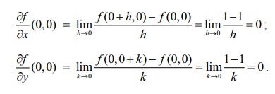
This
completes (i).
Now for
(ii) let us calculate the limit of f as
( x , y) ŌåÆ (0, 0) along the line y = x . Then lim( x , y ) ŌåÆ(0 , 0) f (x
, y) = 0 ; because along the line y = x when x ŌēĀ 0, f ( x , y) = 0 , But f (0, 0) = 1 ŌēĀ 0 ; hence f
cannot be continuous at (0, 0).
Example 8.12
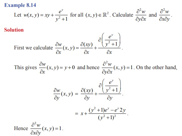
Let F ( x, y ) = x3y + y2x + 7 for all ( x , y) Ōłł ŌäØ2 . Calculate ŌłéF/Ōłéx(ŌłÆ1, 3) and ŌłéF/Ōłéx(ŌłÆ2,1) .
Solution
First we
shall calculate ŌłéF/Ōłéx(x, y),
then we evaluate it at (ŌłÆ1, 3) . As we have already
observed,
we find the derivative with respect to x
holding y as a constant. That is,
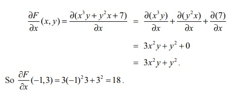
= 3x2y
+ y2 + 0
= 3x2y
+ y2.
So ŌłéF/Ōłéx (ŌłÆ1, 3) = 3(ŌłÆ1)2 3 + 32
= 18 .
Next
similarly we find partial derivative with respect to y.
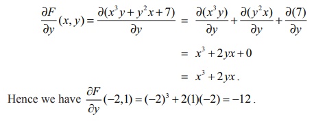
= x3 + 2 yx + 0 = x3 + 2 yx . Hence we have ŌłéF/Ōłéx(ŌłÆ2,1) = (ŌłÆ2 )3 + 2(1)(ŌłÆ2 ) = ŌłÆ12 .
Note
that in the above example ŌłéF/Ōłéx(x , y)
=
3x2y + y2 ,
which is again a function of two variables. So we can take the partial
derivative of this function with respect to x
or y . For instance, if we take G (
x, y ) = 3x2 y +
y2 , then we find ŌłéG/Ōłéx
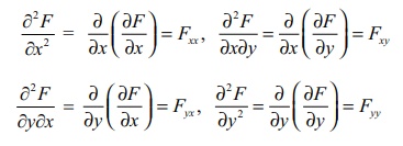
= 6xy . Since G ( x , y) = ŌłéF/Ōłéx , we have ŌłéG/Ōłéx = Ōłé//Ōłéx(ŌłéF/Ōłéx) = 6xy.
We
denote this as Ōłé2F//Ōłé2x ;
which is called the second order partial derivative
of F with respect to x.
Also, ŌłéG/Ōłéy
= 3x2 + 2 y . Since G ( x , y) = ŌłéF/Ōłéy , we have ŌłéG/Ōłéy = Ōłé/Ōłéy(ŌłéF/Ōłéy)
= 3x2 + 2y . We denote this as Ōłé2F / ŌłéyŌłéx
; which is called the mixed partial derivative
of F with respect to x , y . Similarly we can also calculate Ōłé/Ōłéx
(ŌłéF/Ōłéy) = 3x2 + 2y .
Also, if
we differentiate ŌłéF / Ōłéy ( x , y) partially
with respect to y we obtain Ōłé2F
/ Ōłéy2; which is called the second order partial derivatives of F
with respect to y . So for any function
F defined on any subset {(x,y) | a
< x < b, c < y < d} ŌŖé ŌäØ2 we have the following notation :
All the
above are called second order partial derivatives of F . Similarly we can
define higher order partial derivatives. For example,

Next we
shall see more examples on partial differentiation.
Example 8.13
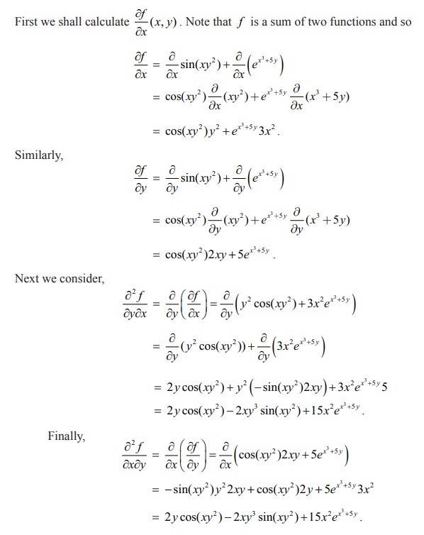
Let f (x, y ) = sin(xy2
) + ex3+5y for all ( x , y) Ōłł
ŌäØ2 . Calculate 
Solution
Note
that we have first used sum rule, then in the next step we have used chain
rule. In the third step, product rule is used. Also, we see that f xy
=
f yx
. Is it a coincidence? or is it always true? Actually, there are functions for
which f xy ŌēĀ f
yx at some points. The
following theorem gives conditions under which f xy =
f yx
.
Theorem 8.1 (ClairautŌĆÖs Theorem)
Suppose that A = {( x, y ) | a < x < b, c < y < d} ŌŖé ŌäØ2, F : A ŌåÆ ŌäØ. If fxy
and f yx exist in A
are continuous in A , then f xy
= f yx in A .
We omit the discussion on the proof at this stage.
Definition 8.9
Let A = { ( x , y ) | a < x b, c < y < d } ŌŖé ŌäØ2. A function u : A ŌåÆ ŌäØ2 is said to be harmonic in A if it satisfies Ōłé2u/Ōłé2x + Ōłé2u/Ōłé2y = 0, ŌłĆ(x , y) Ōłł A . This equation is
called LaplaceŌĆÖs equation.
LaplaceŌĆÖs
equation occurs in the study of many natural phenomena like heat conduction,
electrostatic field, fluid flows etc.
Example 8.15
Let u ( x,
y ) = eŌłÆ2y cos(2x) for all (
x , y) Ōłł
ŌäØ2 . Prove that u is a harmonic function in ŌäØ2 .
Solution
We need to
show that u satisfies the LaplaceŌĆÖs equation
in ŌäØ2 . Observe that ux ( x, y ) = eŌłÆ2 y
(ŌłÆ2)
sin(2x) and hence u xx
(x, y ) = eŌłÆ2 y
(ŌłÆ2)(2)
cos(2x) .
Similarly,
u y
(x, y ) = eŌłÆ2 y
(ŌłÆ2)
cos(2x) and u yy (x, y
) =
( ŌłÆ2)(ŌłÆ2)eŌłÆ2 y
cos(2x) .
Thus, u xx
+
uyy = ŌłÆ4
e ŌłÆ2 y
cos(2x ) +
4e ŌłÆ2 y
cos(2x) =
0.
Related Topics