Chapter: Introduction to the Design and Analysis of Algorithms
Fundamental Data Structures
Fundamental Data Structures
1.
Linear Data Structures
2.
Graphs
3. Trees
4. Sets
and Dictionaries
Since the vast majority of algorithms of
interest operate on data, particular ways of organizing data play a critical
role in the design and analysis of algorithms. A data structure can be defined
as a particular scheme of organizing related data items. The nature of the data
items is dictated by the problem at hand; they can range from elementary data
types (e.g., integers or characters) to data structures (e.g., a
one-dimensional array of one-dimensional arrays is often used for implementing
matrices). There are a few data structures that have proved to be particularly
important for computer algorithms. Since you are undoubtedly familiar with most
if not all of them, just a quick review is provided here.
Linear Data Structures
The two most important elementary data
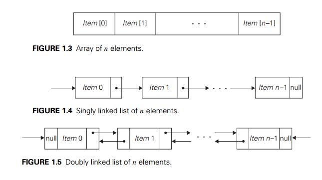
structures are the array and the linked list. A (one-dimensional) array
is a sequence of n items of the same data type that are stored
contiguously in computer memory and made accessible by specifying a value of
the arrayŌĆÖs index (Figure 1.3).
In the majority of cases, the index is an
integer either between 0 and n ŌłÆ 1 (as shown in Figure 1.3) or between 1 and n. Some computer languages allow an array index to range between any
two integer bounds low and high, and some even permit nonnumerical indices to
specify, for example, data items corresponding to the 12 months of the year by
the month names.
Each and every element of an array can be
accessed in the same constant amount of time regardless of where in the array
the element in question is located. This feature positively distinguishes
arrays from linked lists, discussed below.
Arrays are used for implementing a variety of
other data structures. Promi-nent among them is the string, a sequence of
characters from an alphabet termi-nated by a special character indicating the
stringŌĆÖs end. Strings composed of zeros and ones are called binary
strings or bit strings. Strings are indispensable for pro-cessing textual
data, defining computer languages and compiling programs written in them, and
studying abstract computational models. Operations we usually per-form on
strings differ from those we typically perform on other arrays (say, arrays of
numbers). They include computing the string length, comparing two strings to
determine which one precedes the other in lexicographic (i.e., alphabetical) or-der,
and concatenating two strings (forming one string from two given strings by appending
the second to the end of the first).
A linked list is a sequence of zero or
more elements called nodes, each containing two kinds of
information: some data and one or more links called pointers to other nodes
of the linked list. (A special pointer called ŌĆ£nullŌĆØ is used to
indicate the absence of a nodeŌĆÖs successor.) In a singly linked list, each
node except the last one contains a single pointer to the next element (Figure
1.4).
To access a particular node of a linked list, one starts with the
listŌĆÖs first node and traverses the pointer chain until the particular node is
reached. Thus, the time needed to access an element of a singly linked list,
unlike that of an array, depends on where in the list the element is located.
On the positive side, linked lists do
not require any preliminary reservation of the
computer memory, and insertions and deletions can be made quite efficiently in
a linked list by reconnecting a few appropriate pointers.
We can exploit flexibility of the linked list
structure in a variety of ways. For example, it is often convenient to start a
linked list with a special node called the header. This node may contain
information about the linked list itself, such as its current length; it may
also contain, in addition to a pointer to the first element, a pointer to the
linked listŌĆÖs last element.
Another extension is the structure called the doubly
linked list, in which every node, except the first and the last,
contains pointers to both its successor and its predecessor (Figure 1.5).
The array and linked list are two principal
choices in representing a more abstract data structure called a linear list or
simply a list. A list is a finite sequence of data items, i.e., a collection of
data items arranged in a certain linear order. The basic operations performed
on this data structure are searching for, inserting, and deleting an element.
Two special types of lists, stacks and queues,
are particularly important. A stack is a list in which insertions
and deletions can be done only at the end. This end is called the top
because a stack is usually visualized not horizontally but verticallyŌĆöakin to a
stack of plates whose ŌĆ£operationsŌĆØ it mimics very closely. As a result, when
elements are added to (pushed onto) a stack and deleted from (popped off) it,
the structure operates in a ŌĆ£last-inŌĆōfirst-outŌĆØ (LIFO) fashionŌĆö exactly like a
stack of plates if we can add or remove a plate only from the top. Stacks have
a multitude of applications; in particular, they are indispensable for
implementing recursive algorithms.
A queue, on the other hand, is a list
from which elements are deleted from one end of the structure, called the front
(this operation is called dequeue), and new elements are added
to the other end, called the rear (this operation is called enqueue).
Consequently, a queue operates in a ŌĆ£first-inŌĆōfirst-outŌĆØ (FIFO) fashionŌĆöakin to
a queue of customers served by a single teller in a bank. Queues also have many
important applications, including several algorithms for graph problems.
Graphs
As we mentioned in the previous section, a
graph is informally thought of as a collection of points in the plane called
ŌĆ£verticesŌĆØ or ŌĆ£nodes,ŌĆØ some of them connected by line segments called ŌĆ£edgesŌĆØ
or ŌĆ£arcs.ŌĆØ Formally, a graph G = V , E is defined by a pair of two sets: a finite
nonempty set V of items called vertices and a set E of pairs of these items called edges. If these pairs of
vertices are unordered, i.e., a pair of vertices (u, v) is the same as the pair (v, u), we say that the vertices u and v are adjacent to each other and that they
are connected by the undirected edge (u, v). We call
the vertices u and v endpoints of the edge (u, v) and say that u and v are incident to this edge; we also say
that the edge (u, v) is incident to its endpoints u and v. A graph G is called undirected if every edge in it is
undirected.
If a pair of vertices (u, v) is not the same as the pair (v, u), we say that the edge (u, v) is directed from the vertex u, called the edgeŌĆÖs tail, to the vertex v, called the edgeŌĆÖs head. We also say that the edge (u, v) leaves u and enters v. A graph whose every edge is directed is called
directed.
Directed graphs are also called digraphs.
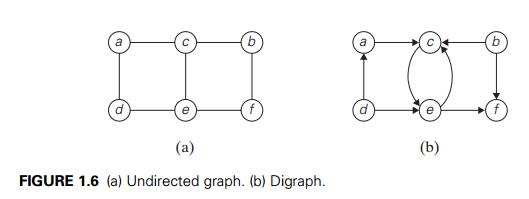
It is normally convenient to label vertices of
a graph or a digraph with letters, integer numbers, or, if an application calls
for it, character strings (Figure 1.6). The graph depicted in Figure 1.6a has
six vertices and seven undirected edges:
V = {a, b,
c, d, e, f }, E = {(a, c), (a, d), (b, c), (b, f ), (c, e), (d,
e), (e, f )}.
The digraph depicted in Figure 1.6b has six
vertices and eight directed edges:
V = {a, b,
c, d, e, f }, E = {(a, c), (b, c), (b, f ), (c, e), (d, a), (d,
e), (e, c), (e, f )}.
Our definition of a graph does not forbid loops,
or edges connecting vertices to themselves. Unless explicitly stated otherwise,
we will consider graphs without loops. Since our definition disallows multiple
edges between the same vertices of an undirected graph, we have the following
inequality for the number of edges |E| possible in an undirected graph with |V | vertices and no loops:
0 Ōēż |E|
Ōēż |V |(|V | ŌłÆ 1)/2.
(We get the largest number of edges in a graph
if there is an edge connecting each of its |V | vertices with all |V | ŌłÆ 1 other vertices. We have to divide product |V |(|V | ŌłÆ 1) by 2, however, because it includes every edge twice.)
A graph with every pair of its vertices
connected by an edge is called complete. A standard notation for
the complete graph with |V | vertices is K|V |. A graph with relatively few possible edges
missing is called dense; a graph with few edges relative to the number of its
vertices is called sparse. Whether we are dealing with a dense or sparse graph may
influence how we choose to represent the graph and, consequently, the running
time of an algorithm being designed or used.
Graph
Representations Graphs
for computer algorithms are usually repre-sented in one of two ways: the adjacency
matrix and adjacency lists. The adjacency matrix of a graph with n vertices
is an
n ├Ś n boolean matrix with one row and one column for each of the
graphŌĆÖs vertices, in which the element in the ith row and the j th column is equal to 1 if there is an edge
from the ith vertex to the j th vertex, and equal to 0 if there is no such
edge. For example, the adjacency matrix for the graph of Figure 1.6a is given
in Figure 1.7a.
Note that the adjacency matrix of an undirected
graph is always symmetric, i.e., A[i, j ] = A[j, i] for every 0 Ōēż i, j Ōēż n ŌłÆ 1 (why?).
The adjacency lists of a graph or a
digraph is a collection of linked lists, one for each vertex, that contain all
the vertices adjacent to the listŌĆÖs vertex (i.e., all the vertices connected to
it by an edge). Usually, such lists start with a header identifying a vertex
for which the list is compiled. For example, Figure 1.7b represents the graph
in Figure 1.6a via its adjacency lists. To put it another way,
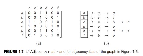
adjacency lists indicate columns of the
adjacency matrix that, for a given vertex, contain 1ŌĆÖs.
If a graph is sparse, the adjacency list
representation may use less space than the corresponding adjacency matrix
despite the extra storage consumed by pointers of the linked lists; the
situation is exactly opposite for dense graphs. In general, which of the two
representations is more convenient depends on the nature of the problem, on the
algorithm used for solving it, and, possibly, on the type of input graph
(sparse or dense).
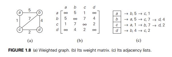
Weighted
Graphs A weighted graph (or
weighted digraph) is a graph (or di-graph) with numbers assigned to its edges.
These numbers are called weights or costs. An interest in
such graphs is motivated by numerous real-world applica-tions, such as finding the
shortest path between two points in a transportation or communication network
or the traveling salesman problem mentioned earlier.
Both principal representations of a graph can
be easily adopted to accommo-date weighted graphs. If a weighted graph is represented
by its adjacency matrix, then its element A[i, j ] will simply contain the weight of the edge
from the ith to the j th vertex if there is such an edge and a
special symbol, e.g., Ōł×, if there is no such edge. Such a matrix is
called the weight matrix or cost matrix. This approach is
illustrated in Figure 1.8b for the weighted graph in Figure 1.8a. (For some
ap-plications, it is more convenient to put 0ŌĆÖs on the main diagonal of the adjacency
matrix.) Adjacency lists for a weighted graph have to include in their nodes
not only the name of an adjacent vertex but also the weight of the
corresponding edge (Figure 1.8c).
Paths
and Cycles Among
the many properties of graphs, two are important for a great number of applications: connectivity and acyclicity.
Both are based on the notion of a path. A path from vertex u to vertex v of a graph G can be defined as a sequence of adjacent
(connected by an edge) vertices that starts with u and ends with v. If all vertices of a path are distinct, the
path is said to be simple. The length of a path is the total number
of vertices in the vertex sequence defining the path minus 1, which is the same
as the number of edges in the path. For example, a, c, b, f is a simple path of length 3 from a to f in the graph in Figure 1.6a, whereas a, c, e, c, b, f is a path (not simple) of length 5 from a to f.
In the case of a directed graph, we are usually
interested in directed paths. A directed path is a sequence of
vertices in which every consecutive pair of the vertices is connected by an
edge directed from the vertex listed first to the vertex listed next. For
example, a, c, e, f is a directed path from a to f in the graph in Figure 1.6b.
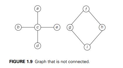
A graph is said to be connected if for every
pair of its vertices u and v there is a path from u to v. If we make a model of a connected graph by
connecting some balls representing the graphŌĆÖs vertices with strings
representing the edges, it will be a single piece. If a graph is not connected,
such a model will consist of several connected pieces that are called connected
components of the graph. Formally, a connected component is a maximal
(not expandable by including another vertex and an edge) connected subgraph2
of a given graph. For example, the graphs in Figures 1.6a and 1.8a are
connected, whereas the graph in Figure 1.9 is not, because there is no path,
for example, from a to f. The graph in Figure 1.9 has two connected
components with vertices {a, b, c, d, e} and {f, g,
h, i}, respectively.
Graphs with several connected components do
happen in real-world appli-cations. A graph representing the Interstate highway
system of the United States would be an example (why?).
It is important to know for many applications
whether or not a graph under consideration has cycles. A cycle is a path of a
positive length that starts and ends at the same vertex and does not traverse
the same edge more than once. For example, f , h, i, g, f is a cycle in the graph in Figure 1.9. A graph
with no cycles is said to be acyclic. We discuss acyclic graphs
in the next subsection.
Trees
A tree (more accurately, a free
tree) is a connected acyclic graph (Figure 1.10a). A graph that has no
cycles but is not necessarily connected is called a forest: each of its
connected components is a tree (Figure 1.10b).
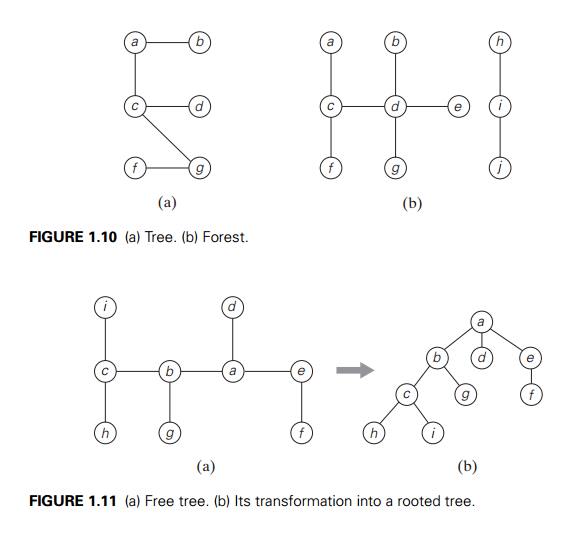
Trees have several important properties other
graphs do not have. In par-ticular, the number of edges in a tree is always one
less than the number of its vertices:
|E| = |V | ŌłÆ 1.
As the graph in Figure 1.9 demonstrates, this
property is necessary but not suffi-cient for a graph to be a tree. However,
for connected graphs it is sufficient and hence provides a convenient way of
checking whether a connected graph has a cycle.
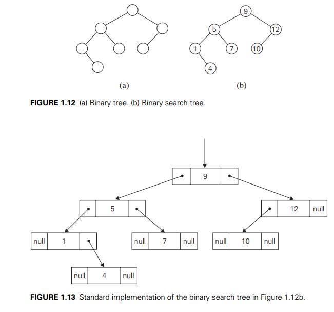
Rooted
Trees Another very important
property of trees is the fact that for every two vertices in a tree, there always exists exactly one simple
path from one of these vertices to the other. This property makes it possible
to select an arbitrary vertex in a free tree and consider it as the root
of the so-called rooted tree. A rooted tree is usually depicted by placing its
root on the top (level 0 of the tree), the vertices adjacent to the root below
it (level 1), the vertices two edges apart from the root still below (level 2),
and so on. Figure 1.11 presents such a transformation from a free tree to a
rooted tree.
Rooted trees play a very important role in
computer science, a much more important one than free trees do; in fact, for
the sake of brevity, they are often referred to as simply ŌĆ£trees.ŌĆØ An obvious
application of trees is for describing hierarchies, from file directories to
organizational charts of enterprises. There are many less obvious applications,
such as implementing dictionaries (see below), efficient access to very large
data sets (Section 7.4), and data encoding (Section 9.4). As we discuss in
Chapter 2, trees also are helpful in analysis of recursive algorithms. To
finish this far-from-complete list of tree applications, we should mention the
so-called state-space trees that underline two important algorithm design
techniques: backtracking and branch-and-bound (Sections 12.1 and 12.2).
For any vertex v in a tree T , all the vertices on the simple path from the
root to that vertex are called ancestors of v. The vertex itself is usually considered its own ancestor; the set
of ancestors that excludes the vertex itself is referred to as the set of proper
ancestors. If (u, v) is the last edge of the simple path from the
root to vertex v (and u = v), u is said to be the parent of v and v is called a child of u; vertices that have the same parent are said to be siblings.
A vertex with no children is called a leaf ; a vertex with at least one
child is called parental. All the vertices for which a vertex v is an ancestor are said to be descendants of v; the proper descendants exclude the vertex v itself.
All the descendants of a vertex v with all the edges connecting them form the subtree of T rooted at that vertex. Thus, for the tree in Figure 1.11b, the
root of the tree is a; vertices d, g, f,
h, and i are leaves, and vertices a, b, e, and c are parental; the parent of b is a; the children of b are c and g; the siblings of b are d and e; and the vertices of the subtree rooted at b are {b, c, g, h, i}.
The depth of a vertex v is the length of the simple path from the root to v. The height of a tree is the length of the longest simple path from
the root to a leaf. For example, the depth of vertex c of the tree in Figure 1.11b is 2, and the height of the tree is 3.
Thus, if we count tree levels top down starting with 0 for the rootŌĆÖs level,
the depth of a vertex is simply its level in the tree, and the treeŌĆÖs height is
the maximum level of its vertices. (You should be alert to the fact that some
authors define the height of a tree as the number of levels in it; this makes
the height of a tree larger by 1 than the height defined as the length of the
longest simple path from the root to a leaf.)
Ordered
Trees An ordered tree is a rooted
tree in which all the children of each vertex
are ordered. It is convenient to assume that in a treeŌĆÖs diagram, all the
children are ordered left to right.
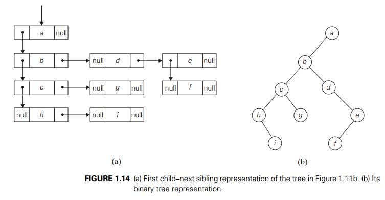
A binary tree can be defined as an
ordered tree in which every vertex has no more than two children and each child
is designated as either a left child or a right child of its
parent; a binary tree may also be empty. An example of a binary tree
is given in Figure 1.12a. The binary tree with its root at the left (right)
child of a vertex in a binary tree is called the left (right)
subtree
of that vertex. Since left and right subtrees are binary trees as well, a
binary tree can also be defined recursively. This makes it possible to solve
many problems involving binary trees by recursive algorithms.
In Figure 1.12b, some numbers are assigned to
vertices of the binary tree in Figure 1.12a. Note that a number assigned to
each parental vertex is larger than all the numbers in its left subtree and
smaller than all the numbers in its right subtree. Such trees are called binary
search trees. Binary trees and binary search trees have a wide variety
of applications in computer science; you will encounter some of them throughout
the book. In particular, binary search trees can be generalized to more general
types of search trees called multiway search trees, which are
indispensable for efficient access to very large data sets.
As you will see later in the book, the
efficiency of most important algorithms for binary search trees and their
extensions depends on the treeŌĆÖs height. There-fore, the following inequalities
for the height h of a binary tree with n nodes are especially important for analysis of such algorithms:
log2 n Ōēż h Ōēż n ŌłÆ 1.
A binary tree is usually implemented for
computing purposes by a collection of nodes corresponding to vertices of the
tree. Each node contains some informa-tion associated with the vertex (its name
or some value assigned to it) and two pointers to the nodes representing the
left child and right child of the vertex, re-spectively. Figure 1.13
illustrates such an implementation for the binary search tree in Figure 1.12b.
A computer representation of an arbitrary
ordered tree can be done by simply providing a parental vertex with the number
of pointers equal to the number of its children. This representation may prove
to be inconvenient if the number of children varies widely among the nodes. We
can avoid this inconvenience by using nodes with just two pointers, as we did
for binary trees. Here, however, the left pointer will point to the first child
of the vertex, and the right pointer will point to its next sibling.
Accordingly, this representation is called the first childŌĆōnext sibling
representation. Thus, all the siblings of a vertex are linked via the
nodesŌĆÖ right pointers in a singly linked list, with the first element
of the list pointed to by the left pointer of their parent. Figure 1.14a
illustrates this representation for the tree in Figure 1.11b. It is not
difficult to see that this representation effectively transforms an ordered
tree into a binary tree said to be associated with the ordered tree. We get
this representation by ŌĆ£rotatingŌĆØ the pointers about 45 degrees clockwise (see
Figure 1.14b).
Sets and Dictionaries
The notion of a set plays a central role in
mathematics. A set can be described as an unordered collection (possibly
empty) of distinct items called elements of the
set. A specific set is defined either by an
explicit listing of its elements (e.g., S = {2, 3, 5, 7}) or by specifying a property that all the setŌĆÖs
elements and only they must satisfy (e.g., S = {n: n is a prime number smaller than 10}). The most
important set operations are: checking membership of a given item in a given
set; finding the union of two sets, which comprises all the elements in either
or both of them; and finding the intersection of two sets, which comprises all
the common elements in the sets.
Sets can be implemented in computer
applications in two ways. The first considers only sets that are subsets of
some large set U, called the universal set.
If set U has n elements, then any subset S of U can be represented by a bit string of size n, called a bit vector, in which the ith element is 1 if and only if the ith element of U is included in set S. Thus, to continue with our example, if U = {1, 2, 3, 4, 5, 6, 7, 8, 9}, then S = {2, 3, 5, 7} is represented by the bit string 011010100. This way of representing sets makes it possible to
implement the standard set operations very fast, but at the expense of
potentially using a large amount of storage.
The second and more common way to represent a
set for computing purposes is to use the list structure to indicate the setŌĆÖs
elements. Of course, this option, too, is feasible only for finite sets;
fortunately, unlike mathematics, this is the kind of sets most computer
applications need. Note, however, the two principal points of distinction
between sets and lists. First, a set cannot contain identical elements; a list
can. This requirement for uniqueness is sometimes circumvented by the
introduction of a multiset, or bag, an unordered collection of
items that are not necessarily distinct. Second, a set is an unordered
collection of items; therefore, changing the order of its elements does not
change the set. A list, defined as an ordered collection of items, is exactly
the opposite. This is an important theoretical distinction, but fortunately it
is not important for many applications. It is also worth mentioning that if a
set is represented by a list, depending on the application at hand, it might be
worth maintaining the list in a sorted order.
In
computing, the operations we need to perform for a set or a multiset most often
are searching for a given item, adding a new item, and deleting an item from
the collection. A data structure that implements these three operations is
called the dictionary. Note the relationship between this data structure
and the problem of searching mentioned in Section 1.3; obviously, we are
dealing here with searching in a dynamic context. Consequently, an efficient
implementation of a dictionary has to strike a compromise between the
efficiency of searching and the efficiencies of the other two operations. There
are quite a few ways a dictionary can be implemented. They range from an
unsophisticated use of arrays (sorted or not) to much more sophisticated
techniques such as hashing and balanced search trees, which we discuss later in
the book.
A number of applications in computing require a
dynamic partition of some n-element set into a collection of disjoint
subsets. After being initialized as a collection of n one-element subsets, the collection is
subjected to a sequence of intermixed union and search operations. This problem
is called the set union problem. We discuss efficient
algorithmic solutions to this problem in Section 9.2, in conjunction with one
of its important applications.
You may have noticed that in our review of
basic data structures we almost al-ways mentioned specific operations that are
typically performed for the structure in question. This intimate relationship
between the data and operations has been recognized by computer scientists for
a long time. It has led them in particular to the idea of an abstract
data type (ADT): a set of abstract objects represent-ing data items with a
collection of operations that can be performed on them. As illustrations of
this notion, reread, say, our definitions of the priority queue and dictionary.
Although abstract data types could be implemented in older procedu-ral
languages such as Pascal (see, e.g., [Aho83]), it is much more convenient to do
this in object-oriented languages such as C++ and Java, which support abstract
data types by means of classes.
Exercises
1.4
Describe
how one can implement each of the following operations on an array so that the
time it takes does not depend on the arrayŌĆÖs size n.
Delete the ith element of an array (1 Ōēż
i Ōēż n).
Delete the ith element of a sorted
array (the remaining array has to stay sorted, of course).
If
you have to solve the searching problem for a list of n numbers, how can you
take advantage of the fact that the list is known to be sorted? Give separate
answers for
lists represented as arrays.
lists represented as linked lists.
a.
Show the stack after each operation of the following sequence that starts with
the empty stack:
push(a), push(b), pop, push(c), push(d), pop
Show
the queue after each operation of the following sequence that starts with the
empty queue:
enqueue(a), enqueue(b), dequeue, enqueue(c),
enqueue(d), dequeue
a.
Let A be the adjacency matrix of an undirected graph. Explain what prop-erty of
the matrix indicates that
the
graph is complete.
the
graph has a loop, i.e., an edge connecting a vertex to itself.
the
graph has an isolated vertex, i.e., a vertex with no edges incident to it.
Answer
the same questions for the adjacency list representation.
Give a detailed description of an algorithm for
transforming a free tree into a tree rooted at a given vertex of the free tree.
6. Prove the inequalities that bracket the
height of a binary tree with n vertices:
log2 n Ōēż
h Ōēż n ŌłÆ 1.
Indicate
how the ADT priority queue can be implemented as
an
(unsorted) array.
a
sorted array.
a
binary search tree.
How
would you implement a dictionary of a reasonably small size n if you knew that
all its elements are distinct (e.g., names of the 50 states of the United
States)? Specify an implementation of each dictionary operation.
For
each of the following applications, indicate the most appropriate data
structure:
answering
telephone calls in the order of their known priorities
sending
backlog orders to customers in the order they have been received
implementing
a calculator for computing simple arithmetical expressions
Anagram
checking Design an algorithm for checking whether two given words are anagrams,
i.e., whether one word can be obtained by permuting the letters of the other.
For example, the words tea and eat are anagrams.
Related Topics