Empirical Analysis of Algorithms

Empirical Analysis of Algorithms

            In few Sections (2.3 and 2.4), we saw how algorithms, both nonrecursive and recursive, can be analyzed mathematically. Though these techniques can be applied success-fully to many simple algorithms, the power of mathematics, even when enhanced with more advanced techniques (see [Sed96], [Pur04], [Gra94], and [Gre07]), is far from limitless. In fact, even some seemingly simple algorithms have proved to be very difficult to analyze with mathematical precision and certainty. As we pointed out in Section 2.1, this is especially true for the average-case analysis.

The principal alternative to the mathematical analysis of an algorithm’s ef-ficiency is its empirical analysis. This approach implies steps spelled out in the following plan.

General Plan for the Empirical Analysis of Algorithm Time Efficiency

            Understand the experiment’s purpose.

            Decide on the efficiency metric M to be measured and the measurement unit (an operation count vs. a time unit).

            Decide on characteristics of the input sample (its range, size, and so on).

            Prepare a program implementing the algorithm (or algorithms) for the exper-imentation.

            Generate a sample of inputs.

            Run the algorithm (or algorithms) on the sample’s inputs and record the data observed.

            Analyze the data obtained.

Let us discuss these steps one at a time. There are several different goals one can pursue in analyzing algorithms empirically. They include checking the accuracy of a theoretical assertion about the algorithm’s efficiency, comparing the efficiency of several algorithms for solving the same problem or different imple-mentations of the same algorithm, developing a hypothesis about the algorithm’s efficiency class, and ascertaining the efficiency of the program implementing the algorithm on a particular machine. Obviously, an experiment’s design should de-pend on the question the experimenter seeks to answer.

In particular, the goal of the experiment should influence, if not dictate, how the algorithm’s efficiency is to be measured. The first alternative is to insert a counter (or counters) into a program implementing the algorithm to count the number of times the algorithm’s basic operation is executed. This is usually a straightforward operation; you should only be mindful of the possibility that the basic operation is executed in several places in the program and that all its executions need to be accounted for. As straightforward as this task usually is, you should always test the modified program to ensure that it works correctly, in terms of both the problem it solves and the counts it yields.

The second alternative is to time the program implementing the algorithm in question. The easiest way to do this is to use a system’s command, such as the time command in UNIX. Alternatively, one can measure the running time of a code

fragment by asking for the system time right before the fragment’s start (t_start) and just after its completion (t_finish), and then computing the difference between the

two (t_finish− t_start).⁷ In C and C++, you can use the function clock for this purpose; in Java, the method currentTimeMillis() in the System class is available.

It is important to keep several facts in mind, however. First, a system’s time is typically not very accurate, and you might get somewhat different results on repeated runs of the same program on the same inputs. An obvious remedy is to make several such measurements and then take their average (or the median) as the sample’s observation point. Second, given the high speed of modern com-puters, the running time may fail to register at all and be reported as zero. The standard trick to overcome this obstacle is to run the program in an extra loop many times, measure the total running time, and then divide it by the number of the loop’s repetitions. Third, on a computer running under a time-sharing system such as UNIX, the reported time may include the time spent by the CPU on other programs, which obviously defeats the purpose of the experiment. Therefore, you should take care to ask the system for the time devoted specifically to execution of your program. (In UNIX, this time is called the “user time,” and it is automatically provided by the time command.)

Thus, measuring the physical running time has several disadvantages, both principal (dependence on a particular machine being the most important of them) and technical, not shared by counting the executions of a basic operation. On the other hand, the physical running time provides very specific information about an algorithm’s performance in a particular computing environment, which can be of more importance to the experimenter than, say, the algorithm’s asymptotic efficiency class. In addition, measuring time spent on different segments of a program can pinpoint a bottleneck in the program’s performance that can be missed by an abstract deliberation about the algorithm’s basic operation. Getting such data—called profiling—is an important resource in the empirical analysis of an algorithm’s running time; the data in question can usually be obtained from the system tools available in most computing environments.

Whether you decide to measure the efficiency by basic operation counting or by time clocking, you will need to decide on a sample of inputs for the experiment. Often, the goal is to use a sample representing a “typical” input; so the challenge is to understand what a “typical” input is. For some classes of algorithms—e.g., for algorithms for the traveling salesman problem that we are going to discuss later in the book—researchers have developed a set of instances they use for benchmark-ing. But much more often than not, an input sample has to be developed by the experimenter. Typically, you will have to make decisions about the sample size (it is sensible to start with a relatively small sample and increase it later if necessary), the range of instance sizes (typically neither trivially small nor excessively large), and a procedure for generating instances in the range chosen. The instance sizes can either adhere to some pattern (e.g., 1000, 2000, 3000, . . . , 10,000 or 500, 1000, 2000, 4000, . . . , 128,000) or be generated randomly within the range chosen.

The principal advantage of size changing according to a pattern is that its impact is easier to analyze. For example, if a sample’s sizes are generated by doubling, you can compute the ratios M(2n)/M(n) of the observed metric M (the count or the time) to see whether the ratios exhibit a behavior typical of algorithms in one of the basic efficiency classes discussed in Section 2.2. The major disadvantage of nonrandom sizes is the possibility that the algorithm under investigation exhibits atypical behavior on the sample chosen. For example, if all the sizes in a sample are even and your algorithm runs much more slowly on odd-size inputs, the empirical results will be quite misleading.

            Another important issue concerning sizes in an experiment’s sample is whether several instances of the same size should be included. If you expect the observed metric to vary considerably on instances of the same size, it would be probably wise to include several instances for every size in the sample. (There are well-developed methods in statistics to help the experimenter make such de-cisions; you will find no shortage of books on this subject.) Of course, if several instances of the same size are included in the sample, the averages or medians of the observed values for each size should be computed and investigated instead of or in addition to individual sample points.

Much more often than not, an empirical analysis requires generating random numbers. Even if you decide to use a pattern for input sizes, you will typically want instances themselves generated randomly. Generating random numbers on a digital computer is known to present a difficult problem because, in principle, the problem can be solved only approximately. This is the reason computer scien-tists prefer to call such numbers pseudorandom. As a practical matter, the easiest and most natural way of getting such numbers is to take advantage of a random number generator available in computer language libraries. Typically, its output will be a value of a (pseudo)random variable uniformly distributed in the interval between 0 and 1. If a different (pseudo)random variable is desired, an appro-priate transformation needs to be made. For example, if x is a continuous ran-dom variable uniformly distributed on the interval 0 ≤ x < 1, the variable y = l+ x(r − l) will be uniformly distributed among the integer values between integers l and r − 1 (l < r).

Alternatively, you can implement one of several known algorithms for gener-ating (pseudo)random numbers. The most widely used and thoroughly studied of such algorithms is the linear congruential method.

ALGORITHM     Random(n, m, seed, a, b)

//Generates a sequence of n pseudorandom numbers according to the linear

            congruential method

//Input: A positive integer n and positive integer parameters m, seed, a, b //Output: A sequence r₁, . . . , r_n of n pseudorandom integers uniformly

            distributed among integer values between 0 and m − 1 //Note: Pseudorandom numbers between 0 and 1 can be obtained

            by treating the integers generated as digits after the decimal point

r₀ ← seed

for i ← 1 to n do

r_i ← (a ∗ r_i−1 + b) mod m

The simplicity of this pseudocode is misleading because the devil lies in the details of choosing the algorithm’s parameters. Here is a partial list of recommen-dations based on the results of a sophisticated mathematical analysis (see [KnuII, pp. 184–185] for details): seed may be chosen arbitrarily and is often set to the current date and time; m should be large and may be conveniently taken as 2^w, where w is the computer’s word size; a should be selected as an integer between 0.01m and 0.99m with no particular pattern in its digits but such that a mod 8 = 5; and the value of b can be chosen as 1.

            The empirical data obtained as the result of an experiment need to be recorded and then presented for an analysis. Data can be presented numerically in a table or graphically in a scatterplot, i.e., by points in a Cartesian coordinate system. It is a good idea to use both these options whenever it is feasible because both methods have their unique strengths and weaknesses.

The principal advantage of tabulated data lies in the opportunity to manip-ulate it easily. For example, one can compute the ratios M(n)/g(n) where g(n) is a candidate to represent the efficiency class of the algorithm in question. If the algorithm is indeed in  (g(n)), most likely these ratios will converge to some pos-itive constant as n gets large. (Note that careless novices sometimes assume that this constant must be 1, which is, of course, incorrect according to the definition of  (g(n)).) Or one can compute the ratios M(2n)/M(n) and see how the running time reacts to doubling of its input size. As we discussed in Section 2.2, such ratios should change only slightly for logarithmic algorithms and most likely converge to 2, 4, and 8 for linear, quadratic, and cubic algorithms, respectively—to name the most obvious and convenient cases.

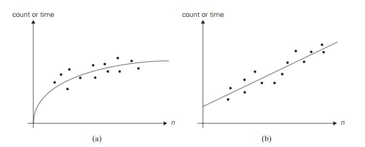
On the other hand, the form of a scatterplot may also help in ascertaining the algorithm’s probable efficiency class. For a logarithmic algorithm, the scat-terplot will have a concave shape (Figure 2.7a); this fact distinguishes it from all the other basic efficiency classes. For a linear algorithm, the points will tend to aggregate around a straight line or, more generally, to be contained between two straight lines (Figure 2.7b). 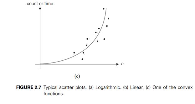Scatterplots of functions in  (n lg n) and  (n²) will have a convex shape (Figure 2.7c), making them difficult to differentiate. A scatterplot of a cubic algorithm will also have a convex shape, but it will show a much more rapid increase in the metric’s values. An exponential algorithm will most probably require a logarithmic scale for the vertical axis, in which the val-ues of log_a M(n) rather than those of M(n) are plotted. (The commonly used logarithm base is 2 or 10.) In such a coordinate system, a scatterplot of a truly exponential algorithm should resemble a linear function because M(n) ≈ caⁿ im-plies log_b M(n) ≈ log_b c + n log_b a, and vice versa.

One of the possible applications of the empirical analysis is to predict the al-gorithm’s performance on an instance not included in the experiment sample. For example, if you observe that the ratios M(n)/g(n) are close to some constant c for the sample instances, it could be sensible to approximate M(n) by the prod-uct cg(n) for other instances, too. This approach should be used with caution, especially for values of n outside the sample range. (Mathematicians call such predictions extrapolation, as opposed to interpolation, which deals with values within the sample range.) Of course, you can try unleashing the standard tech-niques of statistical data analysis and prediction. Note, however, that the majority of such techniques are based on specific probabilistic assumptions that may or may not be valid for the experimental data in question.

            It seems appropriate to end this section by pointing out the basic differ-ences between mathematical and empirical analyses of algorithms. The princi-pal strength of the mathematical analysis is its independence of specific inputs; its principal weakness is its limited applicability, especially for investigating the average-case efficiency. The principal strength of the empirical analysis lies in its applicability to any algorithm, but its results can depend on the particular sample of instances and the computer used in the experiment.

Exercises 2.6

            1. Consider the following well-known sorting algorithm, which is studied later in the book, with a counter inserted to count the number of key comparisons.

ALGORITHM                      SortAnalysis(A[0..n − 1])

//Input: An array A[0..n − 1] of n orderable elements

//Output: The total number of key comparisons made count ← 0

for i ← 1 to n − 1 do

v ← A[i] j ← i − 1

while j ≥ 0 and A[j ] > v do count ← count + 1

A[j + 1] ← A[j ] j ← j − 1

A[j + 1] ← v return count

Is the comparison counter inserted in the right place? If you believe it is, prove it; if you believe it is not, make an appropriate correction.

            2. a. Run the program of Problem 1, with a properly inserted counter (or coun-ters) for the number of key comparisons, on 20 random arrays of sizes 1000, 2000, 3000, . . . , 20,000.

            Analyze the data obtained to form a hypothesis about the algorithm’s average-case efficiency.

            Estimate the number of key comparisons we should expect for a randomly generated array of size 25,000 sorted by the same algorithm.

            3. Repeat Problem 2 by measuring the program’s running time in milliseconds.

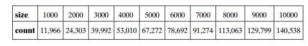
            4. Hypothesize a likely efficiency class of an algorithm based on the following empirical observations of its basic operation’s count:

            5. What scale transformation will make a logarithmic scatterplot look like a linear one?

            6. How can one distinguish a scatterplot for an algorithm in  (lg lg n) from a scatterplot for an algorithm in  (lg n)?

            7. a. Find empirically the largest number of divisions made by Euclid’s algo-rithm for computing gcd(m, n) for 1≤ n ≤ m ≤ 100.

            For each positive integer k, find empirically the smallest pair of integers 1≤ n ≤ m ≤ 100 for which Euclid’s algorithm needs to make k divisions in order to find gcd(m, n).

8. The average-case efficiency of Euclid’s algorithm on inputs of size n can be measured by the average number of divisions D_avg(n) made by the algorithm in computing gcd(n, 1), gcd(n, 2), . . . , gcd(n, n). For example,

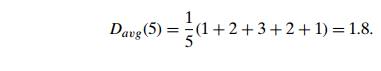
Produce a scatterplot of D_avg(n) and indicate the algorithm’s likely average-case efficiency class.

            9. Run an experiment to ascertain the efficiency class of the sieve of Eratos-thenes (see Section 1.1).

            10. Run a timing experiment for the three algorithms for computing gcd(m, n) presented in Section 1.1.