Mathematical Analysis of Non recursive Algorithms

Mathematical Analysis of Non recursive Algorithms

                        In this section, we systematically apply the general framework outlined in Section 2.1 to analyzing the time efficiency of nonrecursive algorithms. Let us start with a very simple example that demonstrates all the principal steps typically taken in analyzing such algorithms.

EXAMPLE 1 Consider the problem of finding the value of the largest element in a list of n numbers. For simplicity, we assume that the list is implemented as an array. The following is pseudocode of a standard algorithm for solving the problem.

ALGORITHM    MaxElement(A[0..n − 1])

//Determines the value of the largest element in a given array

 //Input: An array A[0..n − 1] of real numbers

//Output: The value of the largest element in A maxval ← A[0]

for i ← 1 to n − 1 do

if A[i] > maxval maxval ← A[i]

return maxval

The obvious measure of an input’s size here is the number of elements in the array, i.e., n. The operations that are going to be executed most often are in the algorithm’s for loop. There are two operations in the loop’s body: the comparison A[i] > maxval and the assignment maxval ← A[i]. Which of these two operations should we consider basic? Since the comparison is executed on each repetition of the loop and the assignment is not, we should consider the comparison to be the algorithm’s basic operation. Note that the number of comparisons will be the same for all arrays of size n; therefore, in terms of this metric, there is no need to distinguish among the worst, average, and best cases here.

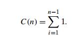
Let us denote C(n) the number of times this comparison is executed and try to find a formula expressing it as a function of size n. The algorithm makes one comparison on each execution of the loop, which is repeated for each value of the loop’s variable i within the bounds 1 and n − 1, inclusive. Therefore, we get the following sum for C(n):

 This is an easy sum to compute because it is nothing other than 1 repeated n − 1 times. Thus,

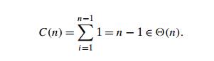
Here is a general plan to follow in analyzing nonrecursive algorithms.

General Plan for Analyzing the Time Efficiency of Nonrecursive Algorithms

Decide on a parameter (or parameters) indicating an input’s size.

Identify the algorithm’s basic operation. (As a rule, it is located in the inner-most loop.)

Check whether the number of times the basic operation is executed depends only on the size of an input. If it also depends on some additional property, the worst-case, average-case, and, if necessary, best-case efficiencies have to be investigated separately.

Set up a sum expressing the number of times the algorithm’s basic operation is executed.

Using standard formulas and rules of sum manipulation, either find a closed-form formula for the count or, at the very least, establish its order of growth.

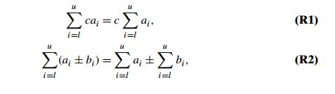
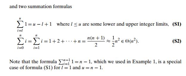
Before proceeding with further examples, you may want to review Appen-dix A, which contains a list of summation formulas and rules that are often useful in analysis of algorithms. In particular, we use especially frequently two basic rules of sum manipulation

EXAMPLE 2 Consider the element uniqueness problem: check whether all the elements in a given array of n elements are distinct. This problem can be solved by the following straightforward algorithm.

ALGORITHM     UniqueElements(A[0..n − 1])

//Determines whether all the elements in a given array are distinct //Input: An array A[0..n − 1]

//Output: Returns “true” if all the elements in A are distinct // and “false” otherwise

for i ← 0 to n − 2 do

for j ← i + 1 to n − 1 do

if A[i] = A[j ] return false return true

The natural measure of the input’s size here is again n, the number of elements in the array. Since the innermost loop contains a single operation (the comparison of two elements), we should consider it as the algorithm’s basic operation. Note, however, that the number of element comparisons depends not only on n but also on whether there are equal elements in the array and, if there are, which array positions they occupy. We will limit our investigation to the worst case only.

By definition, the worst case input is an array for which the number of element comparisons C_worst (n) is the largest among all arrays of size n. An inspection of the innermost loop reveals that there are two kinds of worst-case inputs—inputs for which the algorithm does not exit the loop prematurely: arrays with no equal elements and arrays in which the last two elements are the only pair of equal elements. For such inputs, one comparison is made for each repetition of the innermost loop, i.e., for each value of the loop variable j between its limits i + 1 and n − 1; this is repeated for each value of the outer loop, i.e., for each value of the loop variable i between its limits 0 and n − 2. Accordingly, we get

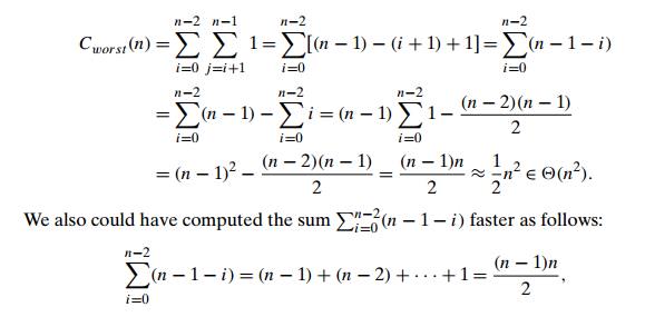
where the last equality is obtained by applying summation formula (S2). Note that this result was perfectly predictable: in the worst case, the algorithm needs to compare all n(n − 1)/2 distinct pairs of its n elements.

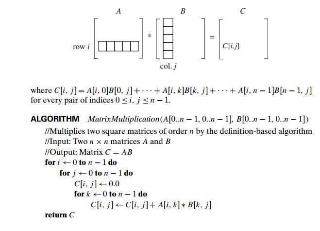
EXAMPLE 3 Given two n × n matrices A and B, find the time efficiency of the definition-based algorithm for computing their product C = AB. By definition, C is an n × n matrix whose elements are computed as the scalar (dot) products of the rows of matrix A and the columns of matrix B:

We measure an input’s size by matrix order n. There are two arithmetical operations in the innermost loop here—multiplication and addition—that, in principle, can compete for designation as the algorithm’s basic operation. Actually, we do not have to choose between them, because on each repetition of the innermost loop each of the two is executed exactly once. So by counting one we automatically count the other. Still, following a well-established tradition, we consider multiplication as the basic operation (see Section 2.1). Let us set up a sum for the total number of multiplications M(n) executed by the algorithm. (Since this count depends only on the size of the input matrices, we do not have to investigate the worst-case, average-case, and best-case efficiencies separately.)

Obviously, there is just one multiplication executed on each repetition of the algorithm’s innermost loop, which is governed by the variable k ranging from the lower bound 0 to the upper bound n − 1. Therefore, the number of multiplications made for every pair of specific values of variables i and j is

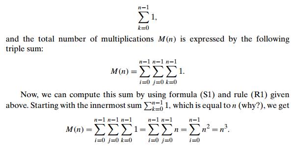
This example is simple enough so that we could get this result without all the summation machinations. How? The algorithm computes n² elements of the product matrix. Each of the product’s elements is computed as the scalar (dot) product of an n-element row of the first matrix and an n-element column of the second matrix, which takes n multiplications. So the total number of multiplica-tions is n ^. n² = n³. (It is this kind of reasoning that we expected you to employ when answering this question in Problem 2 of Exercises 2.1.)

If we now want to estimate the running time of the algorithm on a particular machine, we can do it by the product

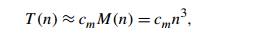
where c_m is the time of one multiplication on the machine in question. We would get a more accurate estimate if we took into account the time spent on the additions, too:

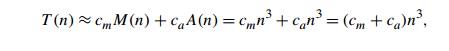
where c_a is the time of one addition. Note that the estimates differ only by their multiplicative constants and not by their order of growth.

You should not have the erroneous impression that the plan outlined above always succeeds in analyzing a nonrecursive algorithm. An irregular change in a loop variable, a sum too complicated to analyze, and the difficulties intrinsic to the average case analysis are just some of the obstacles that can prove to be insur-mountable. These caveats notwithstanding, the plan does work for many simple nonrecursive algorithms, as you will see throughout the subsequent chapters of the book.

As a last example, let us consider an algorithm in which the loop’s variable changes in a different manner from that of the previous examples.

EXAMPLE 4 The following algorithm finds the number of binary digits in the binary representation of a positive decimal integer.

 ALGORITHM                 Binary(n)

//Input: A positive decimal integer n

//Output: The number of binary digits in n’s binary representation count ← 1

while n > 1 do

count ← count + 1 n ← n/2

return count

First, notice that the most frequently executed operation here is not inside the while loop but rather the comparison n > 1 that determines whether the loop’s body will be executed. Since the number of times the comparison will be executed is larger than the number of repetitions of the loop’s body by exactly 1, the choice is not that important.

A more significant feature of this example is the fact that the loop variable takes on only a few values between its lower and upper limits; therefore, we have to use an alternative way of computing the number of times the loop is executed. Since the value of n is about halved on each repetition of the loop, the answer should be about log₂ n. The exact formula for the number of times the comparison n > 1 will be executed is actually log₂ n + 1—the number of bits in the binary representation of n according to formula (2.1). We could also get this answer by applying the analysis technique based on recurrence relations; we discuss this technique in the next section because it is more pertinent to the analysis of recursive algorithms.

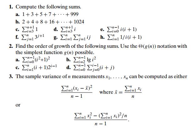
Find and compare the number of divisions, multiplications, and additions/ subtractions (additions and subtractions are usually bunched together) that are required for computing the variance according to each of these formulas.

4. Consider the following algorithm.

ALGORITHM     Mystery(n)

 //Input: A nonnegative integer n S

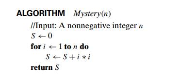
return S

 What does this algorithm compute?

What is its basic operation?

How many times is the basic operation executed?

What is the efficiency class of this algorithm?

Suggest an improvement, or a better algorithm altogether, and indicate its efficiency class. If you cannot do it, try to prove that, in fact, it cannot be done.

5. Consider the following algorithm.

ALGORITHM                      Secret(A[0..n − 1])

//Input: An array A[0..n − 1] of n real numbers minval ← A[0]; maxval ← A[0]

for i ← 1 to n − 1 do

if A[i] < minval minval ← A[i]

if A[i] > maxval maxval ← A[i]

return maxval − minval

Answer questions (a)–(e) of Problem 4 about this algorithm.

6. Consider the following algorithm.

ALGORITHM                      Enigma(A[0..n − 1, 0..n − 1])

//Input: A matrix A[0..n − 1, 0..n − 1] of real numbers for i ← 0 to n − 2 do

for j ← i + 1 to n − 1 do if A[i, j ]  = A[j, i]

return false

return true

Answer questions (a)–(e) of Problem 4 about this algorithm.

                       Improve the implementation of the matrix multiplication algorithm (see Ex-ample 3) by reducing the number of additions made by the algorithm. What effect will this change have on the algorithm’s efficiency?

                       Determine the asymptotic order of growth for the total number of times all the doors are toggled in the locker doors puzzle (Problem 12 in Exercises 1.1).

9 Prove the formula

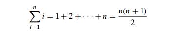
either by mathematical induction or by following the insight of a 10-year-old school boy named Carl Friedrich Gauss (1777–1855) who grew up to become one of the greatest mathematicians of all times.

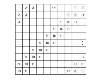
10.Mental arithmetic A 10×10 table is filled with repeating numbers on its diagonals as shown below. Calculate the total sum of the table’s numbers in your head (after [Cra07, Question 1.33]).

                       Consider the following version of an important algorithm that we will study later in the book.

 ALGORITHM     GE(A[0..n − 1, 0..n])

//Input: An n × (n + 1) matrix A[0..n − 1, 0..n] of real numbers for i ← 0 to n − 2 do

for j ← i + 1 to n − 1 do for k ← i to n do

A[j, k] ← A[j, k] − A[i, k] ∗ A[j, i] / A[i, i]

Find the time efficiency class of this algorithm.

What glaring inefficiency does this pseudocode contain and how can it be eliminated to speed the algorithm up?

12. von Neumann’s neighborhood Consider the algorithm that starts with a single square and on each of its n iterations adds new squares all around the outside. How many one-by-one squares are there after n iterations? [Gar99] (In the parlance of cellular automata theory, the answer is the number of cells in the von Neumann neighborhood of range n.) The results for n = 0, 1, and 2 are illustrated below.

13. Page numbering Find the total number of decimal digits needed for num-bering pages in a book of 1000 pages. Assume that the pages are numbered consecutively starting with 1.