Depth-First Search and Breadth-First Search

Depth-First Search and Breadth-First Search

The term “exhaustive search” can also be applied to two very important algorithms that systematically process all vertices and edges of a graph. These two traversal algorithms are depth-first search (DFS) and breadth-first search (BFS). These algorithms have proved to be very useful for many applications involving graphs in artificial intelligence and operations research. In addition, they are indispensable for efficient investigation of fundamental properties of graphs such as connectivity and cycle presence.

Depth-First Search

Depth-first search starts a graph’s traversal at an arbitrary vertex by marking it as visited. On each iteration, the algorithm proceeds to an unvisited vertex that is adjacent to the one it is currently in. (If there are several such vertices, a tie can be resolved arbitrarily. As a practical matter, which of the adjacent unvisited candidates is chosen is dictated by the data structure representing the graph. In our examples, we always break ties by the alphabetical order of the vertices.) This process continues until a dead end—a vertex with no adjacent unvisited vertices— is encountered. At a dead end, the algorithm backs up one edge to the vertex it came from and tries to continue visiting unvisited vertices from there. The algorithm eventually halts after backing up to the starting vertex, with the latter being a dead end. By then, all the vertices in the same connected component as the starting vertex have been visited. If unvisited vertices still remain, the depth-first search must be restarted at any one of them.

It is convenient to use a stack to trace the operation of depth-first search. We push a vertex onto the stack when the vertex is reached for the first time (i.e., the

visit of the vertex starts), and we pop a vertex off the stack when it becomes a dead end (i.e., the visit of the vertex ends).

It is also very useful to accompany a depth-first search traversal by construct-ing the so-called depth-first search forest. The starting vertex of the traversal serves as the root of the first tree in such a forest. Whenever a new unvisited vertex is reached for the first time, it is attached as a child to the vertex from which it is being reached. Such an edge is called a tree edge because the set of all such edges forms a forest. The algorithm may also encounter an edge leading to a previously visited vertex other than its immediate predecessor (i.e., its parent in the tree). 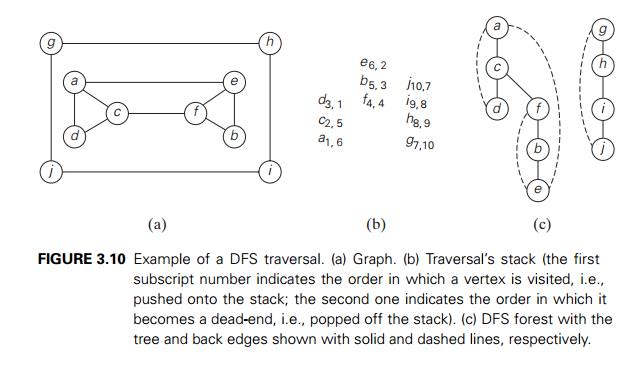Such an edge is called a back edge because it connects a vertex to its ancestor, other than the parent, in the depth-first search forest. Figure 3.10 provides an ex-ample of a depth-first search traversal, with the traversal stack and corresponding depth-first search forest shown as well.

Here is pseudocode of the depth-first search.

ALGORITHM     DFS(G)

//Implements a depth-first search traversal of a given graph //Input: Graph G = V , E

//Output: Graph G with its vertices marked with consecutive integers // in the order they are first encountered by the DFS traversal mark each vertex in V with 0 as a mark of being “unvisited”

count ← 0

for each vertex v in V do if v is marked with 0

dfs(v)

dfs(v)

//visits recursively all the unvisited vertices connected to vertex v //by a path and numbers them in the order they are encountered //via global variable count

count ← count + 1; mark v with count for each vertex w in V adjacent to v do

if w is marked with 0 dfs(w)

The brevity of the DFS pseudocode and the ease with which it can be per-formed by hand may create a wrong impression about the level of sophistication of this algorithm. To appreciate its true power and depth, you should trace the algorithm’s action by looking not at a graph’s diagram but at its adjacency matrix or adjacency lists. (Try it for the graph in Figure 3.10 or a smaller example.)

How efficient is depth-first search? It is not difficult to see that this algorithm is, in fact, quite efficient since it takes just the time proportional to the size of the data structure used for representing the graph in question. Thus, for the adjacency matrix representation, the traversal time is in  (|V |²), and for the adjacency list representation, it is in  (|V | + |E|) where |V | and |E| are the number of the graph’s vertices and edges, respectively.

A DFS forest, which is obtained as a by-product of a DFS traversal, deserves a few comments, too. To begin with, it is not actually a forest. Rather, we can look at it as the given graph with its edges classified by the DFS traversal into two disjoint classes: tree edges and back edges. (No other types are possible for a DFS forest of an undirected graph.) Again, tree edges are edges used by the DFS traversal to reach previously unvisited vertices. If we consider only the edges in this class, we will indeed get a forest. Back edges connect vertices to previously visited vertices other than their immediate predecessors in the traversal. They connect vertices to their ancestors in the forest other than their parents.

A DFS traversal itself and the forest-like representation of the graph it pro-vides have proved to be extremely helpful for the development of efficient al-gorithms for checking many important properties of graphs.³ Note that the DFS yields two orderings of vertices: the order in which the vertices are reached for the first time (pushed onto the stack) and the order in which the vertices become dead ends (popped off the stack). These orders are qualitatively different, and various applications can take advantage of either of them.

Important elementary applications of DFS include checking connectivity and checking acyclicity of a graph. Since dfs halts after visiting all the vertices connected by a path to the starting vertex, checking a graph’s connectivity can be done as follows. Start a DFS traversal at an arbitrary vertex and check, after the algorithm halts, whether all the vertices of the graph will have been vis-ited. If they have, the graph is connected; otherwise, it is not connected. More generally, we can use DFS for identifying connected components of a graph (how?).

As for checking for a cycle presence in a graph, we can take advantage of the graph’s representation in the form of a DFS forest. If the latter does not have back edges, the graph is clearly acyclic. If there is a back edge from some vertex u to its ancestor v (e.g., the back edge from d to a in Figure 3.10c), the graph has a cycle that comprises the path from v to u via a sequence of tree edges in the DFS forest followed by the back edge from u to v.

You will find a few other applications of DFS later in the book, although more sophisticated applications, such as finding articulation points of a graph, are not included. (A vertex of a connected graph is said to be its articulation point if its removal with all edges incident to it breaks the graph into disjoint pieces.)

Breadth-First Search

If depth-first search is a traversal for the brave (the algorithm goes as far from “home” as it can), breadth-first search is a traversal for the cautious. It proceeds in a concentric manner by visiting first all the vertices that are adjacent to a starting vertex, then all unvisited vertices two edges apart from it, and so on, until all the vertices in the same connected component as the starting vertex are visited. If there still remain unvisited vertices, the algorithm has to be restarted at an arbitrary vertex of another connected component of the graph.

It is convenient to use a queue (note the difference from depth-first search!) to trace the operation of breadth-first search. The queue is initialized with the traversal’s starting vertex, which is marked as visited. On each iteration, the algorithm identifies all unvisited vertices that are adjacent to the front vertex, marks them as visited, and adds them to the queue; after that, the front vertex is removed from the queue.

Similarly to a DFS traversal, it is useful to accompany a BFS traversal by con-structing the so-called breadth-first search forest. The traversal’s starting vertex serves as the root of the first tree in such a forest. Whenever a new unvisited vertex is reached for the first time, the vertex is attached as a child to the vertex it is being reached from with an edge called a tree edge. 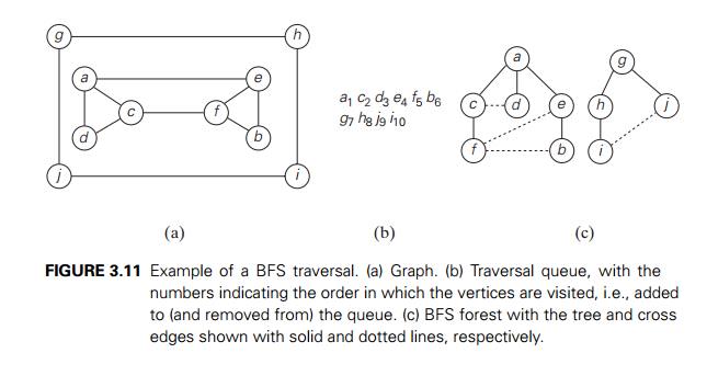If an edge leading to a previously visited vertex other than its immediate predecessor (i.e., its parent in the tree) is encountered, the edge is noted as a cross edge. Figure 3.11 provides an exam-ple of a breadth-first search traversal, with the traversal queue and corresponding breadth-first search forest shown.

Here is pseudocode of the breadth-first search.

ALGORITHM                 BFS(G)

//Implements a breadth-first search traversal of a given graph //Input: Graph G = V , E

//Output: Graph G with its vertices marked with consecutive integers // in the order they are visited by the BFS traversal

mark each vertex in V with 0 as a mark of being “unvisited” count ← 0

for each vertex v in V do if v is marked with 0

bfs(v)

bfs(v)

//visits all the unvisited vertices connected to vertex v

//by a path and numbers them in the order they are visited //via global variable count

count ← count + 1; mark v with count and initialize a queue with v while the queue is not empty do

for each vertex w in V adjacent to the front vertex do if w is marked with 0

count ← count + 1; mark w with count add w to the queue

remove the front vertex from the queue

Breadth-first search has the same efficiency as depth-first search: it is in  (ѳ|V |²) for the adjacency matrix representation and in  ѳ(|V | + |E|) for the adja-cency list representation. Unlike depth-first search, it yields a single ordering of vertices because the queue is a FIFO (first-in first-out) structure and hence the order in which vertices are added to the queue is the same order in which they are removed from it. As to the structure of a BFS forest of an undirected graph, it can also have two kinds of edges: tree edges and cross edges. Tree edges are the ones used to reach previously unvisited vertices. Cross edges connect vertices to those visited before, but, unlike back edges in a DFS tree, they connect vertices either on the same or adjacent levels of a BFS tree.

BFS can be used to check connectivity and acyclicity of a graph, essentially in the same manner as DFS can. It is not applicable, however, for several less straightforward applications such as finding articulation points. On the other hand, it can be helpful in some situations where DFS cannot. For example, BFS can be used for finding a path with the fewest number of edges between two given vertices. To do this, we start a BFS traversal at one of the two vertices and stop it as soon as the other vertex is reached. 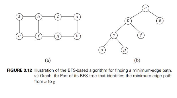The simple path from the root of the BFS tree to the second vertex is the path sought. For example, path a − b − c − g in the graph in Figure 3.12 has the fewest number of edges among all the paths between vertices a and g. Although the correctness of this application appears to stem immediately from the way BFS operates, a mathematical proof of its validity is not quite elementary (see, e.g., [Cor09, Section 22.2]).

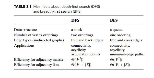
Table 3.1 summarizes the main facts about depth-first search and breadth-first search.

Exercises 3.5

1. Consider the following graph.

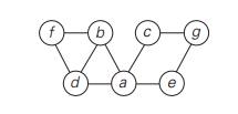
            Write down the adjacency matrix and adjacency lists specifying this graph. (Assume that the matrix rows and columns and vertices in the adjacency lists follow in the alphabetical order of the vertex labels.)

            Starting at vertex a and resolving ties by the vertex alphabetical order, traverse the graph by depth-first search and construct the corresponding depth-first search tree. Give the order in which the vertices were reached for the first time (pushed onto the traversal stack) and the order in which the vertices became dead ends (popped off the stack).

            2. If we define sparse graphs as graphs for which |E| ∈ O(|V |), which implemen-tation of DFS will have a better time efficiency for such graphs, the one that uses the adjacency matrix or the one that uses the adjacency lists?

            3. Let G be a graph with n vertices and m edges.

            True or false: All its DFS forests (for traversals starting at different ver-tices) will have the same number of trees?

            True or false: All its DFS forests will have the same number of tree edges and the same number of back edges?

4. Traverse the graph of Problem 1 by breadth-first search and construct the corresponding breadth-first search tree. Start the traversal at vertex a and resolve ties by the vertex alphabetical order.

        5. Prove that a cross edge in a BFS tree of an undirected graph can connect vertices only on either the same level or on two adjacent levels of a BFS tree.

        6. a. Explain how one can check a graph’s acyclicity by using breadth-first search.

            b. Does either of the two traversals—DFS or BFS—always find a cycle faster than the other? If you answer yes, indicate which of them is better and explain why it is the case; if you answer no, give two examples supporting your answer.

         7. Explain how one can identify connected components of a graph by using

            a depth-first search.

            b breadth-first search.

8. A graph is said to be bipartite if all its vertices can be partitioned into two disjoint subsets X and Y so that every edge connects a vertex in X with a vertex in Y . (One can also say that a graph is bipartite if its vertices can be colored in two colors so that every edge has its vertices colored in different colors; such graphs are also called 2-colorable.) For example, graph (i) is bipartite while graph (ii) is not.

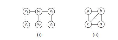
            Design a DFS-based algorithm for checking whether a graph is bipartite.

 Design a BFS-based algorithm for checking whether a graph is bipartite.

            9. Write a program that, for a given graph, outputs:

            vertices of each connected component

            its cycle or a message that the graph is acyclic

            10. One can model a maze by having a vertex for a starting point, a finishing point, dead ends, and all the points in the maze where more than one path can be taken, and then connecting the vertices according to the paths in the maze.

Construct such a graph for the following maze.

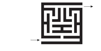
            Which traversal—DFS or BFS—would you use if you found yourself in a maze and why?

   11.  Three Jugs Simeon´ Denis Poisson (1781–1840), a famous French mathemati-cian and physicist, is said to have become interested in mathematics after encountering some version of the following old puzzle. Given an 8-pint jug full of water and two empty jugs of 5- and 3-pint capacity, get exactly 4 pints of water in one of the jugs by completely filling up and/or emptying jugs into others. Solve this puzzle by using breadth-first search.