Where to Sample the Target Population

Where to Sample the Target Population

Sampling errors occur when a sample’s composition is not identical to that of the population from which it is drawn. When the material being sampled is homoge- neous, individual samples can be taken without regard to possible sampling errors. Unfortunately, in most situations the target population is heterogeneous in either time or space. As a result of settling, for example, medications available as oral sus- pensions may have a higher concentration of their active ingredients at the bottom of the container. Before removing a dose (sample), the suspension is shaken to min- imize the effect of this spatial heterogeneity. Clinical samples, such as blood or urine, frequently show a temporal heterogeneity. A patient’s blood glucose level, for instance, will change in response to eating, medication, or exercise. Other systems show both spatial and temporal heterogeneities. The concentration of dissolved O₂ in a lake shows a temporal heterogeneity due to the change in seasons, whereas point sources of pollution may produce a spatial heterogeneity.

When the target population’s heterogeneity is of concern, samples must be ac- quired in a manner that ensures that determinate sampling errors are insignificant. If the target population can be thoroughly homogenized, then samples can be taken without introducing sampling errors. In most cases, however, homogenizing the target population is impracticable. Even more important, homogenization destroys information about the analyte’s spatial or temporal distribution within the target population.

Random Sampling 

The ideal sampling plan provides an unbiased estimate of the target population’s properties. This requirement is satisfied if the sample is collected at random from the target population.3 Despite its apparent simplicity, a true ran- dom sample is difficult to obtain. Haphazard sampling, in which samples are col- lected without a sampling plan, is not random and may reflect an analyst’s uninten- tional biases. 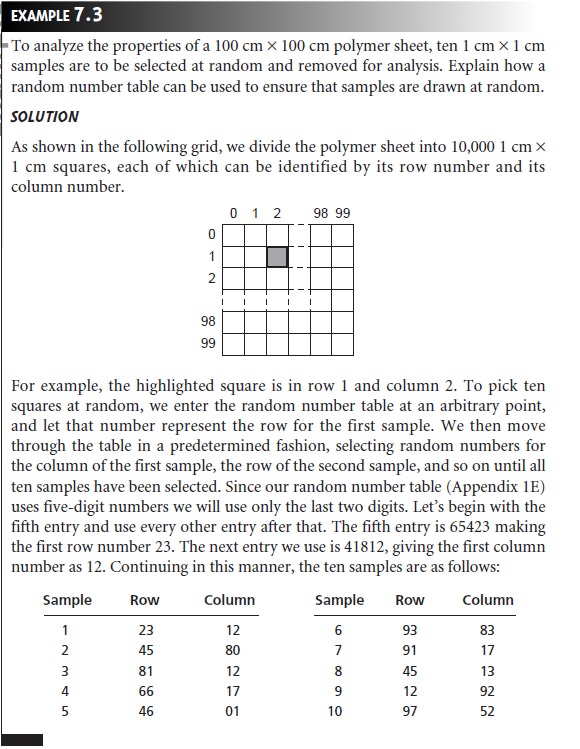The best method for ensuring the collection of a random sample is to divide the target population into equal units, assign a unique number to each unit, and use a random number table (Appendix 1E) to select the units from which to sample. Example 7.3 shows how this is accomplished.

A randomly collected sample makes no assumptions about the target popula- tion, making it the least biased approach to sampling. On the other hand, random sampling requires more time and expense than other sampling methods since a greater number of samples are needed to characterize the target population.

Judgmental Sampling 

The opposite of random sampling is selective, or judg- mental sampling, in which we use available information about the target popula- tion to help select samples. Because assumptions about the target population are included in the sampling plan, judgmental sampling is more biased than random sampling; however, fewer samples are required. Judgmental sampling is common when we wish to limit the number of independent variables influencing the re- sults of an analysis. For example, a researcher studying the bioaccumulation of polychlorinated biphenyls (PCBs) in fish may choose to exclude fish that are too small or that appear diseased. Judgmental sampling is also encountered in many protocols in which the sample to be collected is specifically defined by the regula- tory agency.

Systematic Sampling

Random sampling and judgmental sampling represent ex- tremes in bias and the number of samples needed to accurately characterize the tar- get population. Systematic sampling falls in between these extremes. In systematic sampling the target population is sampled at regular intervals in space or time. 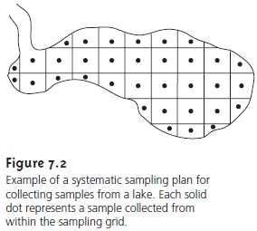For a system exhibiting a spatial heterogeneity, such as the distribution of dissolved O₂ in a lake, samples can be systematically collected by dividing the system into discrete units using a two- or three-dimensional grid pattern (Figure 7.2). Samples are collected from the center of each unit, or at the intersection of grid lines. When a heterogeneity is time-dependent, as is common in clinical studies, samples are drawn at regular intervals.

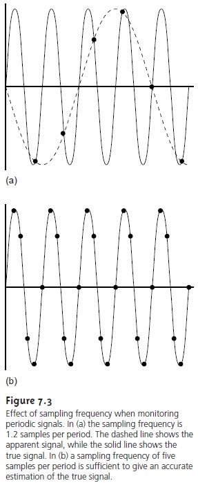
When a target population’s spatial or temporal heterogeneity shows a periodic trend, a systematic sampling leads to a significant bias if samples are not collected frequently enough. This is a common problem when sampling electronic signals, in which case the problem is known as alias- ing. Consider, for example, a signal consisting of a simple sine wave. Fig- ure 7.3a shows how an insufficient sampling frequency underestimates the signal’s true frequency.

According to the Nyquist theorem, to determine a periodic signal’s true fre- quency, we must sample the signal at a rate that is at least twice its frequency (Fig- ure 7.3b); that is, the signal must be sampled at least twice during a single cycle or period. When samples are collected at an interval of ∆t, the highest frequency that can be accurately monitored has a frequency of (2 ∆t)–1. For example, if samples are collected every hour, the highest frequency that we can monitor is 0.5 h–1, or a peri- odic cycle lasting 2 h. A signal with a cycling period of less than 2 h (a frequency of more than 0.5 h–1) cannot be monitored. Ideally, the sampling frequency should be at least three to four times that of the highest frequency signal of interest. Thus, if an hourly periodic cycle is of interest, samples should be collected at least every 15–20 min.

Systematic–Judgmental Sampling 

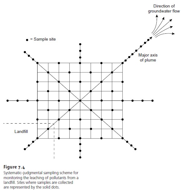
Combinations of the three primary approaches to sampling are also possible.4 One such combination is systematic–judgmental sampling, which is encountered in environmental studies when a spatial or tempo-ral distribution of pollutants is anticipated. For example, a plume of waste leaching from a landfill can reasonably be expected to move in the same di- rection as the flow of groundwater. The systematic–judgmental sampling plan shown in Figure 7.4 includes a rectangular grid for systematic sampling and linear transects extending the sampling along the plume’s suspected major and minor axes.

Stratified Sampling 

Another combination of the three primary approaches to sampling is judgmental–random, or stratified sampling. Many target populations are conveniently subdivided into distinct units, or strata. For example, in determining the concentration of particulate Pb in urban air, the target population can be subdivided by particle size. In this case samples can be collected in two ways. In a random sampling, differences in the strata are ignored, and individual samples are collected at random from the entire target population. In a stratified sampling the target population is divided into strata, and random samples are collected from within each stratum. Strata are analyzed separately, and their respective means are pooled to give an overall mean for the target population.

The advantage of stratified sampling is that the composition of each stra- tum is often more homogeneous than that of the entire target population. When true, the sampling variance for each stratum is less than that when the target population is treated as a single unit. As a result, the overall sampling variance for stratified sampling is always at least as good as, and often better than, that obtained by simple random sampling.

Convenience Sampling 

One additional method of sampling deserves brief mention. In convenience sampling, sample sites are selected using criteria other than minimizing sampling error and sampling variance. In a survey of groundwater quality, for example, samples can be collected by drilling wells at randomly selected sites, or by making use of existing wells. The latter method is usually the preferred choice. In this case, cost, expedience, and accessibility are the primary factors used in selecting sam- pling sites.