The calculation of limits

Limits

The calculation of limits

The notion of a limit, which we will discuss extensively in this chapter, plays a central role in calculus and in much of modern mathematics. However, although mathematics dates back over three thousand years, limits were not really understood until the monumental work of the great French mathematician Augustin – Louis Cauchy and Karl Weierstrass in the nineteenth century, the age of rigour in mathematics.

In this section we define limit and show how limits can be calculated.

Illustration 9.1

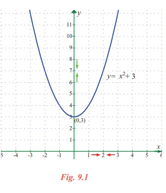
We begin by looking at the function y = f (x ) = x2 + 3 . Note that f  is a function from R→ R  .

Let us investigate the behaviour of this function near x = 2. We can use two sets of x values : one set that approaches 2 from the left (values less than 2) and one set that approaches 2 from the right (values greater than 2) as shown in the table.

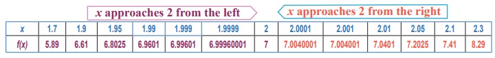
It appears from the table that as x gets close to x = 2, f(x) = x2 + 3 gets close to 7. This is not surprising since if we now calculate f(x) at x = 2, we obtain f(2) = 22 + 3 = 7.

In order to guess at this limit, we didn’t have to evaluate x2 + 3 at x = 2.

That is, as x approaches 2 from either the left (values lower than 2) or right (values higher than

2) the functional values f(x) are approaching 7 from either side; that is, when x is near 2, f(x) is near 7. The above situation is described in a condensed form:

The value 7 is the left limit of f(x) as x approaches 2 from the left as well as 7 is the right limit of  f(x) as x approaches 2 from the right and write :

f (x)→7 as x →2- and f (x ) → 7 as x→2+

or

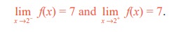
Note also that lim x→2− f(x) = 7 = lim x→2+ f(x). The common value is written as lim x →2  f(x) = 7.

We also observe that the limit is a definite real number. Here, definiteness means that lim x→2− f(x) and lim x→2+  f(x) are the same and lim x→2 f(x) = lim x→2- f(x) = lim x→2+ f(x) is a unique real number.

The figure in Fig. 9.1 explains the geometrical significance of the above discussion of the behaviour of f(x) = x2 + 3 as x → 2.

Illustration 9.2

Next, let us look at the rational function f(x) =

The domain of this function is R \ {-4}. Although f(- 4) is not defined, nonetheless, f(x) can be calculated for any value of x near - 4 because the symbol 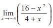says that we consider values of x that are close to - 4 but not equal to - 4. The table below gives the values of f(x) for values of x that approach - 4.

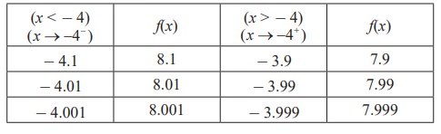
For x ≠ - 4, f(x) can be simplified by cancellation :

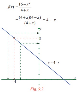
As seen in Fig.9.2, the graph of f(x) is essentially the graph of y = 4 - x with the exception that the graph of f has a hole (puncture) at the point that corresponds to x = - 4. As x gets closer and closer to - 4, represented by the two arrow heads on the x-axis, the two arrow heads on the y-axis simultaneously get closer and closer to the number 8.

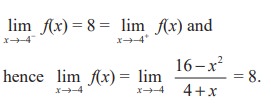
Here, note that

In Illustration 9.2, note that the function is not defined at x = −4 and yet f(x) appears to be approaching a limit as x approaches - 4. This often happens, and it is important to realise that the existence or non-existence of f(x) at x = −4 has no bearing on the existence of the limit of f(x) as x approaches −4 .

Illustration 9.3

Now let us consider a function different from Illustrations 9.1 and 9.2.

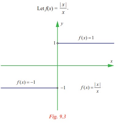
x = 0  does not belong to the domain of this function, R\ {0}. Look at the graph of this function. From the graph one can see that for positive values of x,

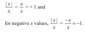
This means that no matter how close x  gets to 0 (in a small neighbourhood of 0), there will be both positive and negative x values that yield f(x) = 1 and f(x) = - 1.

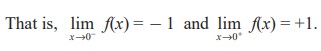
This means that the limit does not exist. Of course, for any other value of x, there is a limit.

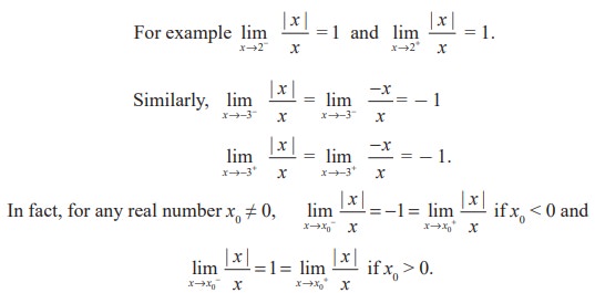
We call the attention of the reader to observe the differences reflected in Illustrations 9.1 to 9.3. In Illustration 9.1, the function f(x) = x2 + 3 is defined at x = 2. i.e., 2 belongs to the domain of f namely = (-∞, ∞). In Illustration 9.2, the function is not defined at x = - 4. In the former case we say the limit, lim x→2f(x) exists as x gets closer and closer to 2 to mean that x→2-f(x) and lim x→2+ f(x) stand for a unique real number. In the later case, although it is not defined at x = - 4, lim x→−4 f(x) exist as x gets closer and closer to - 4. In Illustration 9.3, lim x→0 |x|/x does not exist to mean that the one sided limits are different as x gets sufficiently close to 0. In the light of these observations we have the intuitive notion of limit as in

Definition 9.1

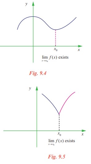
Let I be an open interval containing x0 ∈ R. Let f : I → R. Then we say that the limit of f(x) is L, as x approaches x0 [symbollically written as lim x →x0 f (x ) = L ], if, whenever x becomes sufficiently close to x0 from either side with , x ≠ x0 f (x) gets sufficiently close to L.

The following (Fig 9.4 and 9.5) graphs depict the above narrations.