Continuity - Differential Calculus

Continuity

One of the chief features in the behaviour of functions is the property known as continuity. It reflects mathematically the general trait of many phenomena observed by us in nature. For instance, we speak of the continuous expansion of a rod on heating, of the continuous growth of an organism, of a continuous flow, or a continuous variation of atmospheric temperature etc.

The idea of continuity of a function stems from the geometric notion of “no breaks in a graph”. In fact, the name itself derives from the Latin continuere, “to hang together”. Nevertheless, to identify continuity with “no breaks in a graph” or “a hanging together” has serious drawbacks, at least from the point of view of applying the concept to the analysis of functions. Accordingly, a premature use of the graph to gain insight into the meaning of continuity is advised against as gravely misleading. However, we will realise later that for functions with interval domains, continuity means essentially that the graph may be traced without lifting the point of the pencil.

The proper and effective way of attitude which allows us to put the concept to work is to correlate continuity with limit. Loosely speaking, to possess the property of continuity will mean “to have a favourable limit”. In order to formulate the concept of continuity in terms of limit we must focus our attention at a point. Both continuity and limit are primarily concepts defined at a point, but continuity acquires a global character in a pointwise way.

For motivation, consider the following physical situation. A thermometer T measures T temperatures along a given hot wire L.

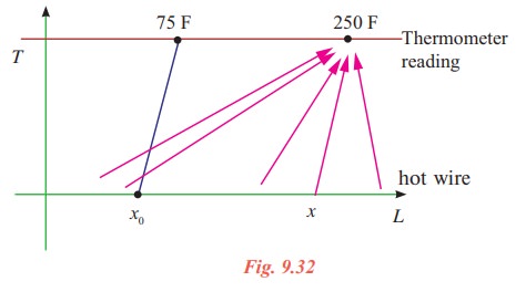
To each point x on the hot wire L is assigned a temperature readings t(x) on thermometer, T. Suppose, to fix ideas, the temperature recordings are observed to be the same, 250°F, as one moves along the wire L until a point x0 is reached on L.

Then suppose that at x0 the temperature drops suddenly to near room temperature, say 75°F, as if an insulation were at x0. But, beyond x0 suppose readings of 250°F are again observed. In function notation we are assuming that

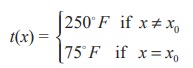
Thus the point x0 stands out as singular point (“singular” means “special” or “unusual”). Analyzing the range of temperature readings, we should say that the approach of x to x0 had no bearing on the approach of the corresponding t(x) values to t(x0). Briefly, a jump occurs at x0. Thus we would be led to say that the temperature function “lacks continuity at x0”. For, we would have expected t(x0) to be 250°F since the x values neighbouring x0 showed t(x) = 250°F. We now abstract the notion of continuity, and demand that images be “close” when pre-images are “close”. In our example the points on the hot wire were the pre-images, while the temperature readings there were the corresponding images.

The students should reflect on the intuitive idea of continuity by considering instead the contrasting idea of lack of continuity, or more simply “discontinuity” as manifested in every day experiences of abrupt changes which could be headed “then suddenly!”. A few that come readily to mind are listed below along with functions which correspond as mathematical models:

1) Switching on a light : light intensity as a function of time.

2) Collision of a vehicle : Velocity as a function of time.

3) Switching off a radio : Sound intensity as a function of time.

4) Busting of a balloon: Radius as a function of air input.

5) Breaking of a string : Tension as a function of length.

6) Cost of postage : Postage as a function of weight.

7) Income tax : Tax-rate as a function of taxable income.

8) Age count in years : Age in whole years as a function of time.

9) Cost of insurance premium : Premium as a function of age.

Actually, examples (1) - (5) are not quite accurate. For example, light intensity has a transparent but continuous passage from zero luminosity to positive luminosity. Indeed, nature appears to abhor discontinuity. On the other hand, (6) - (9) are in fact discontinuous and really show jumps at certain points.

Students are advised to relate the mathematical definition of continuity corresponds closely with the meaning of the word continuity in everyday language. A continuous process is one that takes place gradually, without interruption or abrupt change. That is, there are no holes, jumps or gaps. Following figure identifies three values of x at which the graph of a function f is not continuous. At all other points in the interval (a, b), the graph of f is uninterrupted and continuous.

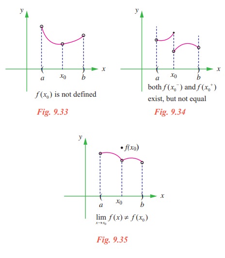
Looking at the above graphs (9.33 to 9.35), three conditions exist for which the graph of f is not continuous at x = x0.

It appears that continuity at x = x0 can be destroyed by any one of the following three conditions:

(1) The function is not defined at x = x0.

(2) The limit of f(x) does not exist at x = x0.

(3) The limit of f(x) exists at x = x0, but, it is not equal to f(x0).

Now let us look at the illustrative examples

Illustration 9.6

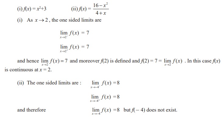
Note that although lim x→−4 f (x) exists, the function value at - 4, namely f(- 4) is not defined. Thus the existence of lim x→−4 f (x) has no bearing on the existence of f(- 4).

Now we formally define continuity as in

Definition 9.7

Let I be an open interval in R containing x0. Let f : I → R. Then f is said to be continuous at x0 if it is defined in a neighbourhood of this point and if the limit of this function, as the independent variable x tends to x0, exists and is equal to the value of the function at x = x0.

Thus three requirements have to be satisfied for the continuity of a function y = f(x) at x = x0 :

(i) f(x) must be defined in a neighbourhood of x0 (i.e., f (x0 ) exists);

(ii) limx →x0 f (x) exists ;

(iii) f(x0) = limx →x0 f (x) .

The condition (iii) can be reformulated as limx →0 [ f (x0+ ∆x ) − f (x0)] = 0  and the continuity of f at x0 can be restated as follows :

Definition 9.8

A function y = f(x) is said to be continuous at a point x0 (or at x = x0) if it is defined in some neighbourhood of x0 and if lim∆x→0 [f (x0 + ∆x ) - f (x0)] = 0 .

The condition (iii) can also be put in the form lim x → x0 f (x ) = f ( lim x →x0 x ) . Thus, if the symbol of the limit and the symbol of the function can be interchanged, the function is continuous at the limiting value of the argument.