Tree Search

TREE SEARCH

Many problems can be solved using a tree search. As a simple example, consider the traveling salesperson problem, or TSP. In TSP, a salesperson is given a list of cities she needs to visit and a cost for traveling between each pair of cities. Her problem is to visit each city once, returning to her hometown, and she must do this with the least possible cost. A route that starts in her hometown, visits each city once and returns to her hometown is called a tour; thus, the TSP is to find a minimum-cost tour.

Unfortunately, TSP is what’s known as an NP-complete problem. From a practi-cal standpoint, this means that there is no algorithm known for solving it that, in all cases, is significantly better than exhaustive search. Exhaustive search means exam-ining all possible solutions to the problem and choosing the best. The number of possible solutions to TSP grows exponentially as the number of cities is increased. For example, if we add one additional city to an n-city problem, we’ll increase the number of possible solutions by a factor of n-1. Thus, although there are only six possible solutions to a four-city problem, there are 4 x 6 = 24 to a five-city problem, 5x 24 = 120 to a six-city problem, 6 x 120 = 720 to a seven-city problem, and so on. In fact, a 100-city problem has far more possible solutions than the number of atoms in the universe!

Furthermore, if we could find a solution to TSP that’s significantly better in all cases than exhaustive search, then there are literally hundreds of other very hard problems for which we could find fast solutions. Not only is there no known solution to TSP that is better in all cases than exhaustive search, it’s very unlikely that we’ll find one.

So how can we solve TSP? There are a number of clever solutions. However, let’s take a look at an especially simple one. It’s a very simple form of tree search. The idea is that in searching for solutions, we build a tree. The leaves of the tree correspond to tours, and the other tree nodes correspond to “partial” tours—routes that have visited some, but not all, of the cities.

Each node of the tree has an associated cost, that is, the cost of the partial tour. We can use this to eliminate some nodes of the tree. Thus, we want to keep track of the cost of the best tour so far, and, if we find a partial tour or node of the tree that couldn’t possibly lead to a less expensive complete tour, we shouldn’t bother searching the children of that node (see Figures 6.9 and 6.10).

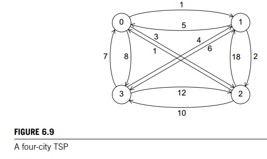
In Figure 6.9 we’ve represented a four-city TSP as a labeled, directed graph. A graph (not to be confused with a graph in calculus) is a collection of vertices and edges or line segments joining pairs of vertices. In a directed graph or digraph, the edges are oriented—one end of each edge is the tail, and the other is the head. A graph or digraph is labeled if the vertices and/or edges have labels. In our example, the vertices of the digraph correspond to the cities in an instance of the TSP, the edges correspond to routes between the cities, and the labels on the edges correspond to the costs of the routes. For example, there’s a cost of 1 to go from city 0 to city 1 and a cost of 5 to go from city 1 to city 0.

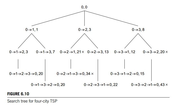
If we choose vertex 0 as the salesperson’s home city, then the initial partial tour consists only of vertex 0, and since we’ve gone nowhere, it’s cost is 0. Thus, the root of the tree in Figure 6.10 has the partial tour consisting only of the vertex 0 with cost 0. From 0 we can first visit 1, 2, or 3, giving us three two-city partial tours with costs 1, 3, and 8, respectively. In Figure 6.10 this gives us three chil-dren of the root. Continuing, we get six three-city partial tours, and since there are

only four cities, once we’ve chosen three of the cities, we know what the complete tour is.

Now, to find a least-cost tour, we should search the tree. There are many ways to do this, but one of the most commonly used is called depth-first search. In depth-first search, we probe as deeply as we can into the tree. After we’ve either reached a leaf or found a tree node that can’t possibly lead to a least-cost tour, we back up to the deepest “ancestor” tree node with unvisited children, and probe one of its children as deeply as possible.

In our example, we’ll start at the root, and branch left until we reach the leaf labeled

0 -> 1  -> 2  -> 3  -> 0, Cost 20.

Then we back up to the tree node labeled 0 ! 1, since it is the deepest ancestor node with unvisited children, and we’ll branch down to get to the leaf labeled

0  -> 1  -> 3  -> 2  -> 0, Cost 20.

Continuing, we’ll back up to the root and branch down to the node labeled 0 ! 2. When we visit its child, labeled

0  -> 2  -> 1, Cost 21,

we’ll go no further in this subtree, since we’ve already found a complete tour with cost less than 21. We’ll back up to 0 ! 2 and branch down to its remaining unvisited child. Continuing in this fashion, we eventually find the least-cost tour

0  -> 3  -> 1  -> 2  -> 0, Cost 15.