Parallelizing the reduced solver using MPI

Parallelizing the reduced solver using MPI

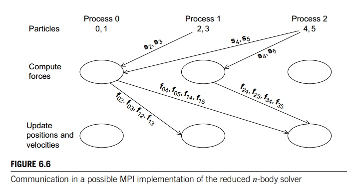
The “obvious” implementation of the reduced algorithm is likely to be extremely complicated. Before computing the forces, each process will need to gather a subset of the positions, and after the computation of the forces, each process will need to scatter some of the individual forces it has computed and add the forces it receives. Figure 6.6 shows the communications that would take place if we had three processes, six particles, and used a block partitioning of the particles among the processes. Not suprisingly, the communications are even more complex when we use a cyclic distribution (see Exercise 6.13). Certainly it would be possible to implement these communications. However, unless the implementation were very carefully done, it would probably be very slow.

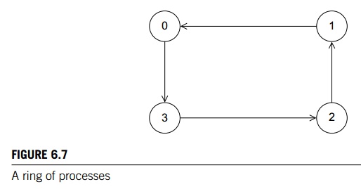
Fortunately, there’s a much simpler alternative that uses a communication struc-ture that is sometimes called a ring pass. In a ring pass, we imagine the processes

as being interconnected in a ring (see Figure 6.7). Process 0 communicates directly with processes 1 and comm._sz -1, process 1 communicates with processes 0 and 2, and so on. The communication in a ring pass takes place in phases, and during each phase each process sends data to its “lower-ranked” neighbor, and receives data from its “higher-ranked” neighbor. Thus, 0 will send to comm sz 1 and receive from 1. 1 will send to 0 and receive from 2, and so on. In general, process q will send to process (q − 1 + comm._sz)%comm sz and receive from process (q + 1)%comm_sz.

By repeatedly sending and receiving data using this ring structure, we can arrange that each process has access to the positions of all the particles. During the first phase, each process will send the positions of its assigned particles to its “lower-ranked” neighbor and receive the positions of the particles assigned to its higher-ranked neigh-bor. 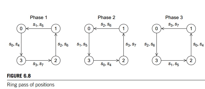During the next phase, each process will forward the positions it received in the first phase. This process continues through comm sz 1 phases until each process has received the positions of all of the particles. Figure 6.8 shows the three phases if there are four processes and eight particles that have been cyclically distributed.

Of course, the virtue of the reduced algorithm is that we don’t need to compute all of the inter-particle forces since f_kq = -  f_qk, for every pair of particles q and k. To see

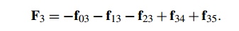
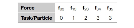
how to exploit this, first observe that using the reduced algorithm, the interparticle forces can be divided into those that are added into and those that are subtracted from the total forces on the particle. For example, if we have six particles, then the reduced algorithm will compute the force on particle 3 as

The key to understanding the ring pass computation of the forces is to observe that the interparticle forces that are subtracted are computed by another task/particle, while the forces that are added are computed by the owning task/particle. Thus, the computations of the interparticle forces on particle 3 are assigned as follows:

So, suppose that for our ring pass, instead of simply passing loc_n = n/comm_sz  positions, we also pass loc_n forces. Then in each phase, a process can 

1. compute interparticle forces resulting from interaction between its assigned particles and the particles whose positions it has received, and

2. once an interparticle force has been computed, the process can add the force into a local array of forces corresponding to its particles, and it can subtract the interparticle force from the received array of forces.

See, for example, [15, 34] for further details and alternatives.

Let’s take a look at how the computation would proceed when we have four par-ticles, two processes, and we’re using a cyclic distribution of the particles among the processes (see Table 6.4). We’re calling the arrays that store the local positions and local forces loc pos and loc forces, respectively. These are not communicated among the processes. The arrays that are communicated among the processes are tmp pos and tmp forces.

Before the ring pass can begin, both arrays storing positions are initialized with the positions of the local particles, and the arrays storing the forces are set to 0. Before the ring pass begins, each process computes those forces that are due to interaction

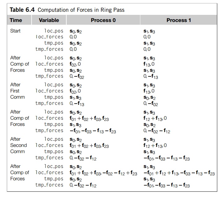
among its assigned particles. Process 0 computes f₀₂ and process 1 computes f₁₃. These values are added into the appropriate locations in loc forces and subtracted from the appropriate locations in tmp forces.

Now, the two processes exchange tmp pos and tmp forces and compute the forces due to interaction among their local particles and the received particles. In the reduced algorithm, the lower ranked task/particle carries out the computation. Process 0 computes f₀₁, f₀₃, and f₂₃, while process 1 computes f₁₂. As before, the newly computed forces are added into the appropriate locations in loc_forces and subtracted from the appropriate locations in tmp_forces.

To complete the algorithm, we need to exchange the tmp arrays one final time.¹ Once each process has received the updated tmp forces, it can carry out a simple vector sum

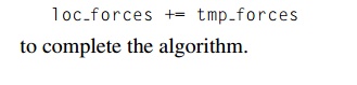
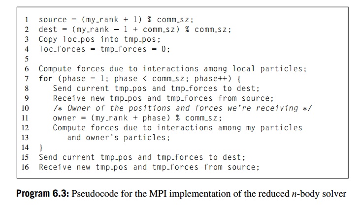
Thus, we can implement the computation of the forces in the reduced algorithm using a ring pass with the pseudocode shown in Program 6.3. Recall that using MPI_Send and MPI_Recv for the send-receive pairs in Lines 8 and 9 and 15 and 16 is unsafe in MPI parlance, since they can hang if the system doesn’t provide sufficient buffering. In this setting, recall that MPI provides MPI_Sendrecv and MPI_Sendrecv_replace. Since we’re using the same memory for both the outgoing and the incoming data, we can use MPI_Sendrecv_replace.

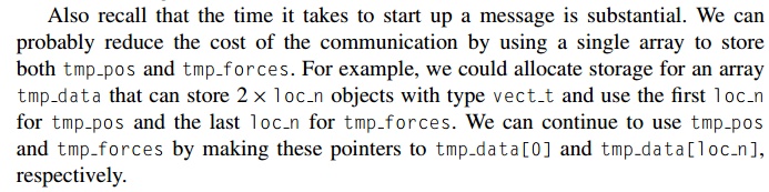
The principal difficulty in implementing the actual computation of the forces in Lines 12 and 13 lies in determining whether the current process should compute the force resulting from the interaction of a particle q assigned to it and a particle r whose position it has received. If we recall the reduced algorithm (Program 6.1), we see that task/particle q is responsible for computing f_qr if and only if q < r. However, the arrays loc_pos and tmp_pos (or a larger array containing tmp_pos and tmp_forces) use local subscripts, not global subscripts. That is, when we access an element of (say) loc pos, the subscript we use will lie in the range 0, 1, …, loc_n-1, not 0, 1, … , n-1; so, if we try to implement the force interaction with the following pseudocode, we’ll run into (at least) a couple of problems:

The first, and most obvious, is that masses is a global array and we’re using local subscripts to access its elements. The second is that the relative sizes of loc_part1 and loc_part2 don’t tell us whether we should compute the force due to their inter-action. We need to use global subscripts to determine this. For example, if we have four particles and two processes, and the preceding code is being run by process 0, then when loc_part1 = 0, the inner loop will skip loc_part2 = 0 and start with loc_part2 = 1; however, if we’re using a cyclic distribution, loc_part1 = 0 corre-sponds to global particle 0 and loc_part2 = 0 corresponds to global particle 1, and we should compute the force resulting from interaction between these two particles.

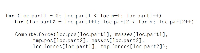
Clearly, the problem is that we shouldn’t be using local particle indexes, but rather we should be using global particle indexes. Thus, using a cyclic distribution of the particles, we could modify our code so that the loops also iterate through global particle indexes:

The function Global_to_local should convert a global particle index into a local par-ticle index, and the function Compute_force should compute the force resulting from the interaction of two particles. We already know how to implement Compute_force. See Exercises 6.15 and 6.16 for the other two functions.